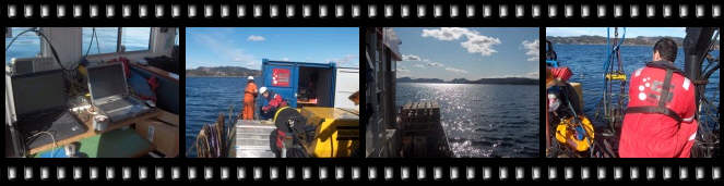
Time Coded Impulse Seismic Technique
|
| Item | Description |
Specifications etc. |
||
|---|---|---|---|---|
| 1 | Mini-streamer, two channels |
|
||
| 2 | Seismic recorder |
|
||
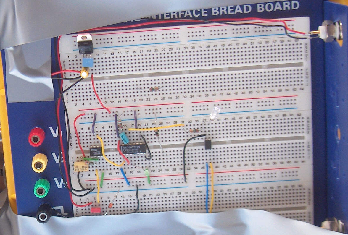
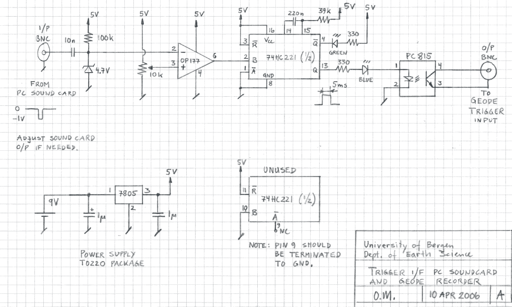
| 3 | Interface PC soundcard O/P and GEODE trigger I/P.
|
|
||
| 4 | GPS connected to GEODE data collecting laptop.
|
|
||
| 5 | GPS used for differential correction |
Used a Garmin GPS-35. Unfortunately, logging of GPS stopped after a short while, for unknown reasons. Will be investigated further. |
3. Test sequence overview (5 April 2006 - B.A.)
| Test # |
Description | Setup
Note: Streamer offset measured between vessel stern and center of first hydrophone group in streamer. LACS positioned approx. 5 m forward from stern, on port side. |
FFID range (called fldr in trace headers)e |
Recording parameters | Raw nav data files |
|---|---|---|---|---|---|
| 1 | LACS far field signature test
Sequence 1 test Sequence 2 test Sequence 1 and 2 test |
|
FFID1000-1195
FFID1196-1205
FFID1206-1216 FFID1217-1228 |
|
Here |
| 2 | LACS as seismic source
Sequence type 1 LEG1 |
|
FFID1229-1287 (logging towards starting point of LEG1)
FFID1288-1440 (LEG1) |
|
-"- |
| 3 | LACS as seismic source
Sequence type 1 and 2 LEG2-a1 |
|
FFID1441-1451 (logging towards starting point of LEG2-a
FFID 1452-1491 (LEG2-a) LACS misfires |
|
-"- |
| 4 | LACS as seismic source
Sequence type 1 and 2 LEG2-a2 |
|
FFID1492-1545(LEG2-a2)
LACS misfires |
|
-"- |
| 4 | LACS as seismic source
Fixed firing rate:0.476 Hz. LEG2-b |
|
FFID1546-1811 |
|
-"- |
| 5 | LACS as seismic source
Sequence type 1 and 2 LEG3 |
|
FFID1812-1968 |
|
-"- |
| 5 | Noise measurement |
|
FFID1969-1978 |
|
-"- |
4. Nav data
4.1 Processing
Raw navdata is here.Navdata is not merged with seismic data (into SEG-Y trace headers). Instead, GPS info associated with each recording is placed in separate file, with GPS info in alternating lines; e.g.:
$GPGGA,091614,6028.0945,N,00514.6330,E,1,10,1.2, - Received at 09:16:49.21 for File 1166
 FFID    1166 (Stack  1, Shot Loc: 0 Meters) 09:16:14.00 04/05/2006   66 KBytes SAVED IN 1166.SGY
$GPGGA,091619,6028.0945,N,00514.6326,E,1,10,1.2, - Received at 09:16:54.31 for File 1167
 FFID    1167 (Stack  1, Shot Loc: 0 Meters) 09:16:19.00 04/05/2006   62 KBytes SAVED IN 1166.SGY
We need to extract Recording Number - called Shotpoint = SP from now - and time, latitude (lat) , longitude (lon) from these files, and also convert lon/lat to UTM Easting/Northing (these fields are highlighted).
Conversion between lat/lon and UTM: Download this Python library http://www.pygps.org/LatLongUTMconversion-1.1.tar.gz.
Unpack it, and run "python setup.py install" as root. In order to build Python modules you must first install 'python-devel'. In SUSE: Yast -> Install and remove software -> Select filter: "Package Groups" -> Development -> Languages -> Python. There you will find "python-devel".
This python script extracts & converts the needed parameters. Input nav data file is given as command line parameter. Output to stdout, so just redirect to file to save output.
To process all *.log files in a directory write the following. Processed files with have the extension ".extract" added to the filename.
for FILE in `ls *.log`; do echo $FILE; ../software/navdata-processing.py $FILE > $FILE.extract; doneThen merge all processed nav data files into one file called "navdata.txt", also sorting by SP, by typing:
cat *.extract | sort > navdata.txt
4.2 Plotting
Have used Generic Mapping Tools (GMT) to make shotpoint maps.Here is example map in png format (click to enlarge).
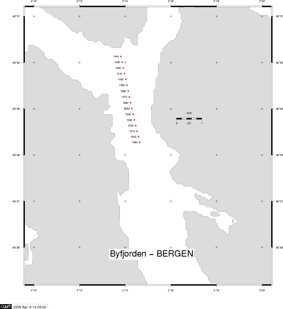
Example SP map (click to enlarge).
Example scripts:
- Bash script to make map above
- Script to plot far-field signature test position
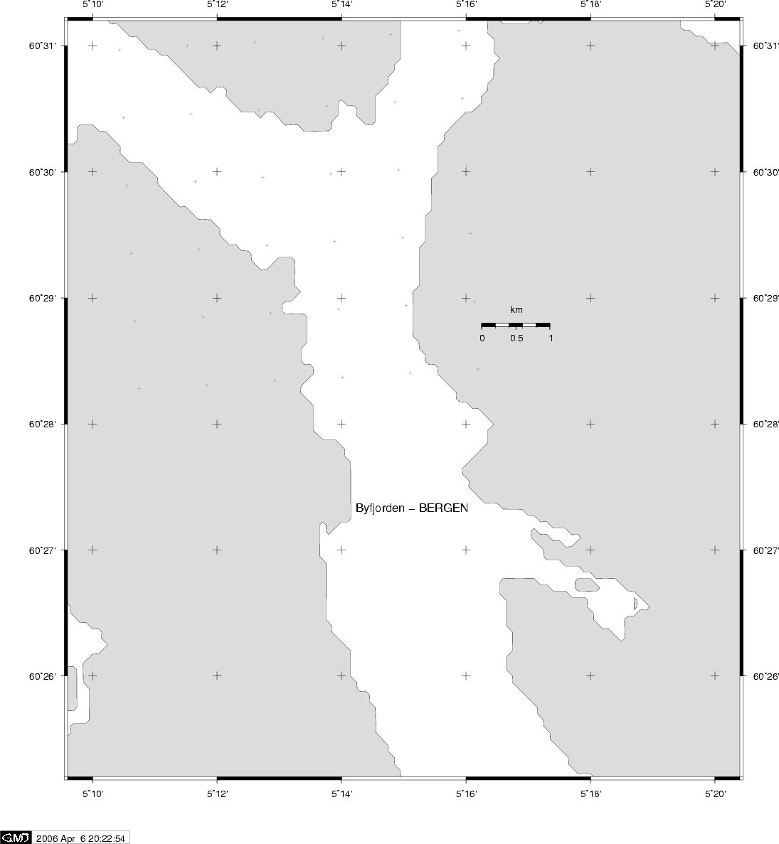
- Trial with UTM grid markers included (1x1 km grid cell size, must be improved). Must first generate UTM grid
points by this Python script.
PNG result is here.
PNG, JPG: Use "convert", which is part of ImageMagick. Output filename extension determines output format.
The -density option determines size (in pixels) of output image.
convert -rotate 90 -trim -antialias -density 120x120 SP-plot-with-UTM-grid.ps SP-plot-with-UTM-grid.pngPDF: Use "ps2pdf", which is part of GMT:
ps2pdf SP-plot-with-UTM-grid.ps SP-plot-with-UTM-grid.pdf
5. Seismic data
Data is in SEG-Y format.- Here's an overview of SEG-Yformat
- The SEG-Y format specification from SEG:
5.1 Importing SEG-Y data to Seismic Unix
In the following we will use the far-field LACS signature test. Data is in 1166.sgy:segyread tape=1166.sgy endian=0 conv=1 | segyclean > 1166.suConvert all SEG-Y files in a directory:
for FILE in `ls *.sgy`; do echo $FILE; segyread file=$FILE conv=1 endian=0 | segyclean | > ${FILE%.*}.su; done
${FILE%.*} is a so-called "string operation" in Bash; it strips off existing file extension ".sgy", so we can replace it by
".su".Parameters:
- conv=1 : According to SEG-Y standard, floating point samples should be in IBM format. Modern PCs use IEEE 754 floating point format, so setting conv=1 will convert samples from IBM to IEEE floating point format (here is some background information on problems caused by mix-up of these formats).
- endian=0: PCs are little-endian machines, so this option should be set to zero.
5.2 Viewing trace header information
First check which trace header parameter fields are in use, and their min/max values, by the surange command:olem@linux:~/www/Naxys/test-week-14-2006/data> surange < 1166.su 180 traces: fldr=(1166,1195) tracf=(1,6) trid=1 nvs=1 nhs=1 scalco=1 gx=(0,5) counit=1 ns=2500 dt=1000 year=6 day=95 hour=9 minute=(16,18) sec=(4,59) timbas=1Here's a list of all trace header parameters. In this particular file the fldr (=SP) goes from 1166 to 1195, and tracf from 1 to 6 (most likely 6 channels were recorded by mistake - should only be 4 - but it's easy to discard ch. 5 and 6, see later).
Use suxedit to investigate individual trace headers, and also "plot" each sample:
olem@linux:~/www/Naxys/test-week-14-2006/data> suxedit < 1166.su

suxedit: ! examine only (no header editing from STDIN)

180 traces in input file
 fldr=1195 tracf=6 trid=1 nvs=1 nhs=1 scalco=1
 gx=5 counit=1 ns=2500 dt=1000 year=6 day=95
 hour=9 minute=18 sec=39 timbas=1
> p
    1 -1.3893e+00                     --------|
    2 -2.0331e+00                 ------------|
    3  1.5508e+00                             |++++++++
    4  4.5063e+00                             |+++++++++++++++++++++++++
    5  2.1204e+00                             |+++++++++++
    6  2.2197e+00                             |++++++++++++
    7  3.6537e-01                             |++
    8 -2.5042e+00              ---------------|
    9  1.0019e+00                             |+++++
   10  3.3873e+00                             |+++++++++++++++++++
   11  1.7798e+00                             |++++++++++
   12 -7.7628e-01                        -----|
   13 -5.1471e+00-----------------------------|
   14 -2.3701e+00               --------------|
   15  4.5092e-01                             |++
   16 -3.1452e+00           ------------------|
   17 -1.2180e+00                      -------|
   18 -2.1906e+00                -------------|
   19 -4.8839e+00 ----------------------------|
>
5.3 Selecting specific traces from a SU data file
The "suwin" command selects specific traces from a data file, based on criteria that is entered on the command line. All examples refers to file 1166.su mentioned above.| Selection no. | You want to: | Write this: |
|---|---|---|
| 1 | Select all 6 traces in last shot in 1166.su and display as wiggle plot. |
suwind key=fldr min=1195 max=1195 < 1166.su | suxwigb |
| 2 | Select trace 4 (far-field hydrophone) in last shot. |
suwind key=fldr min=1195 max=1195 < 1166.su | suwind key=tracf min=4 max=4 | suxwigb |
| 3 | As no. 2, but with bandpass filter. |
suwind key=fldr min=1195 max=1195 < 1166.su | suwind key=tracf min=4 max=4 |\ sufilter f=5,10,200,400 | suxwigb |
| 4 | Select trace 4 (far-field hydrophone) from all traces, and dump to file. |
suwind key=tracf min=4 max=4 < 1166.su > 1166-farfield.su |
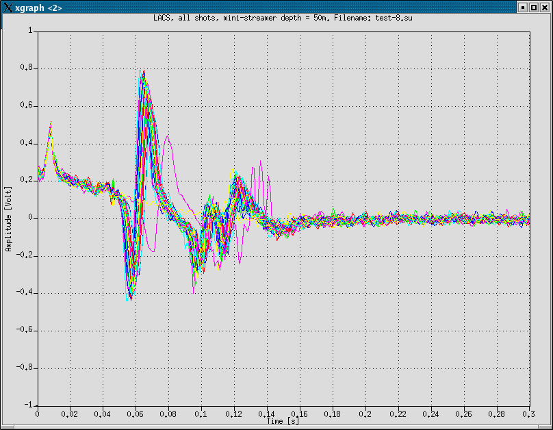
| 5 | Select trace 4 (far-field hydrophone), apply band-pass filter and show using suxgraph. |
suwind key=tracf min=4 max=4 < 1166.su | sufilter f=5,10,200,400 | suxgraph style=normal |
| 6 | Select trace 4 (far-field hydrophone) in first shot, convert to ASCII floats. |
suwind key=fldr min=1166 max=1166 < 1166.su |suwind key=tracf min=4 max=4 |\ sustrip outpar=/dev/null | b2a n1=1 outpar=/dev/null > 1166-SP1166-ch4.txt |
| 7 | Select trace 3 and 4 (near- and far-field hydrophone) in first shot, convert to ASCII floats. |
suwind key=fldr min=1166 max=1166 < 1166.su |suwind key=tracf min=3 max=4 |\ sustrip outpar=/dev/null | b2a n1=2 outpar=/dev/null > 1166-SP1166-ch3+4.txt |
| 8 | Show Gabor spectrogram of trace 4 in first shot. Press <CTRL>+H to change colour palette. |
suwind key=fldr min=1166 max=1166 < 1166.su | suwind key=tracf min=4 max=4 |\ sugabor | suximage |
| 9 | Show frequency spectrum of trace 4 in first shot. Maximize, then drag to zoom area. |
suwind key=fldr min=1166 max=1166 < 1166.su | suwind key=tracf min=4 max=4 |\ suspecfx | suxgraph style=normal |
| 10 | Extract ch 1-4 from each recording, from all SEG-Y files, and export as ASCII floats (4 columns) - one file for each recording. Will also
convert all SEG-Y files to Seismic Unix format. ASCII floats filename example:
1166.su.SP_1170_ch_1+2+3+4.txt
|
This is a Python script. Download from here. |
NOTE: For diagram annotations, grids, axis text and headings in Seismic Unix plots - see examples below.
6. Data preview
We will just show some results from the LACS far-field signature test (single shot). All these plots made with Seismic Unix.
| Thumbnail image - click to enlarge | Script | Comments |
|---|---|---|
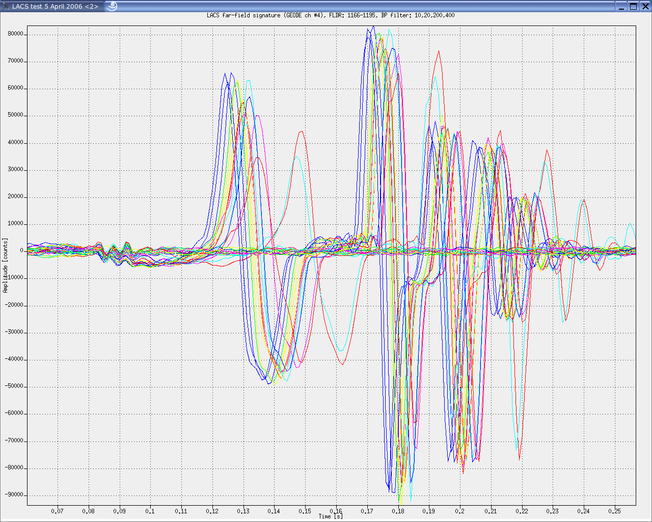 Fig. 6.1: Far-field signature, FLDR 1166-1195, BP filter: 10,20,200,400 |
./software/plot-ff-test.sh |
|
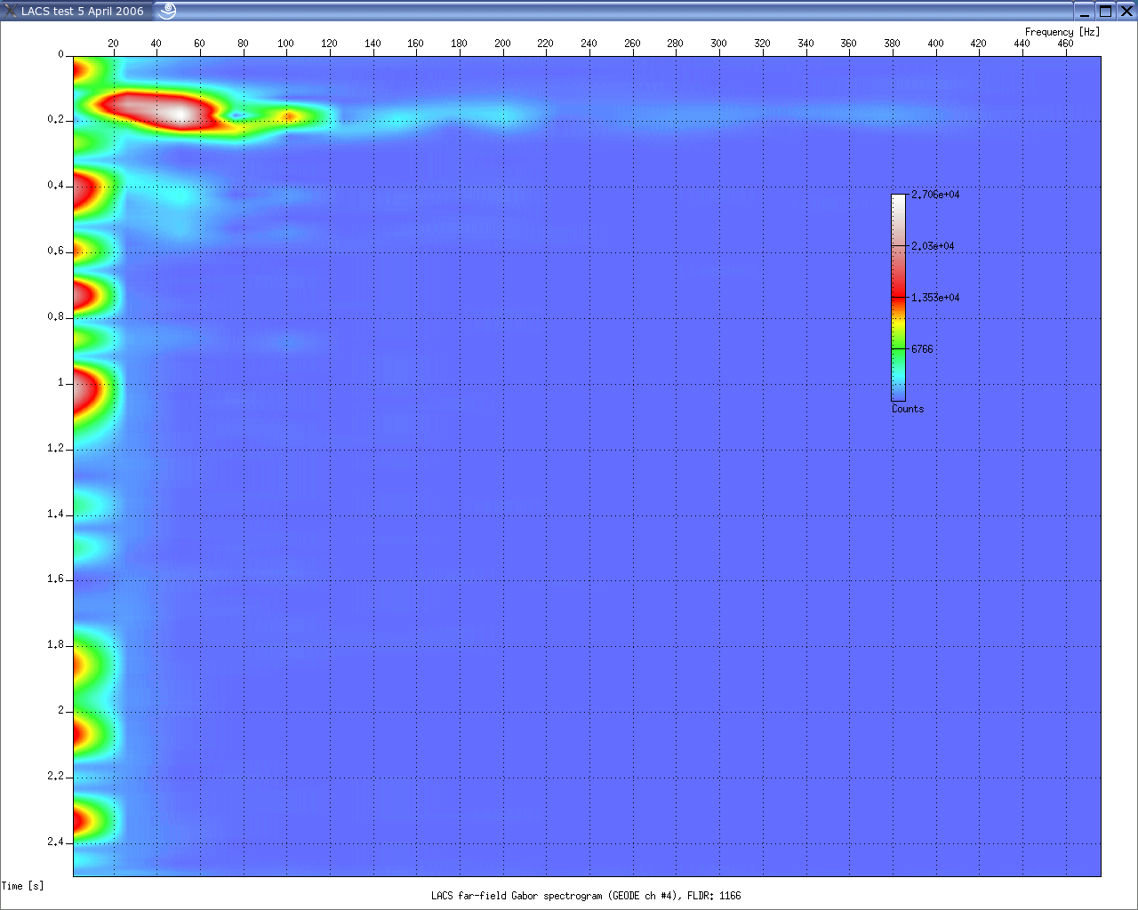 Fig. 6.2: Far-field hydrophone, Gabor spectrogram, FLDR=1166 |
./software/plot-gabor-ff-test.sh | |
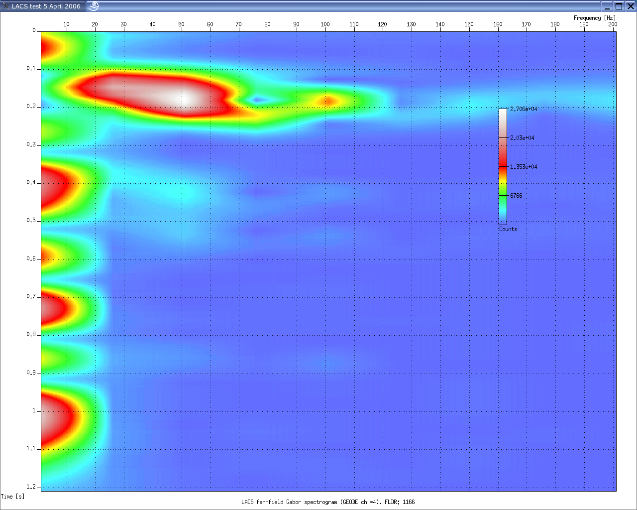 Fig. 6.3: Detail of far-field hydrophone, Gabor spectrogram, FLDR=1166 |
./software/plot-gabor-ff-test.sh |