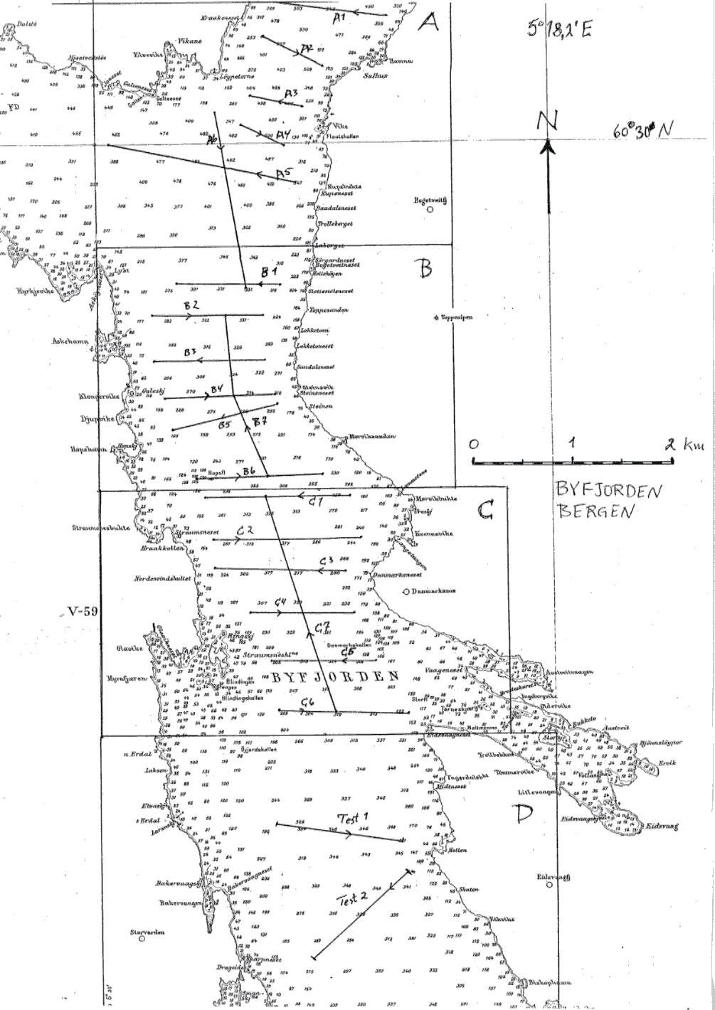
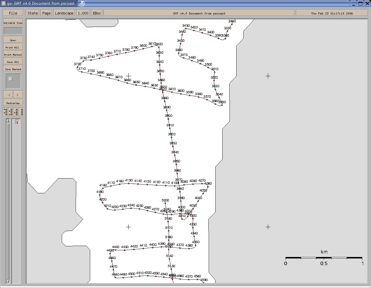
1. Planned lines, vessel

Byfjorden area, Bergen. Click to enlarge.

Institute of Marine Research / UiB R/V "Hans Brattstrm" - link to description.

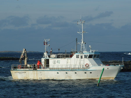
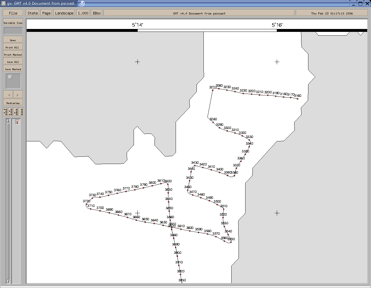
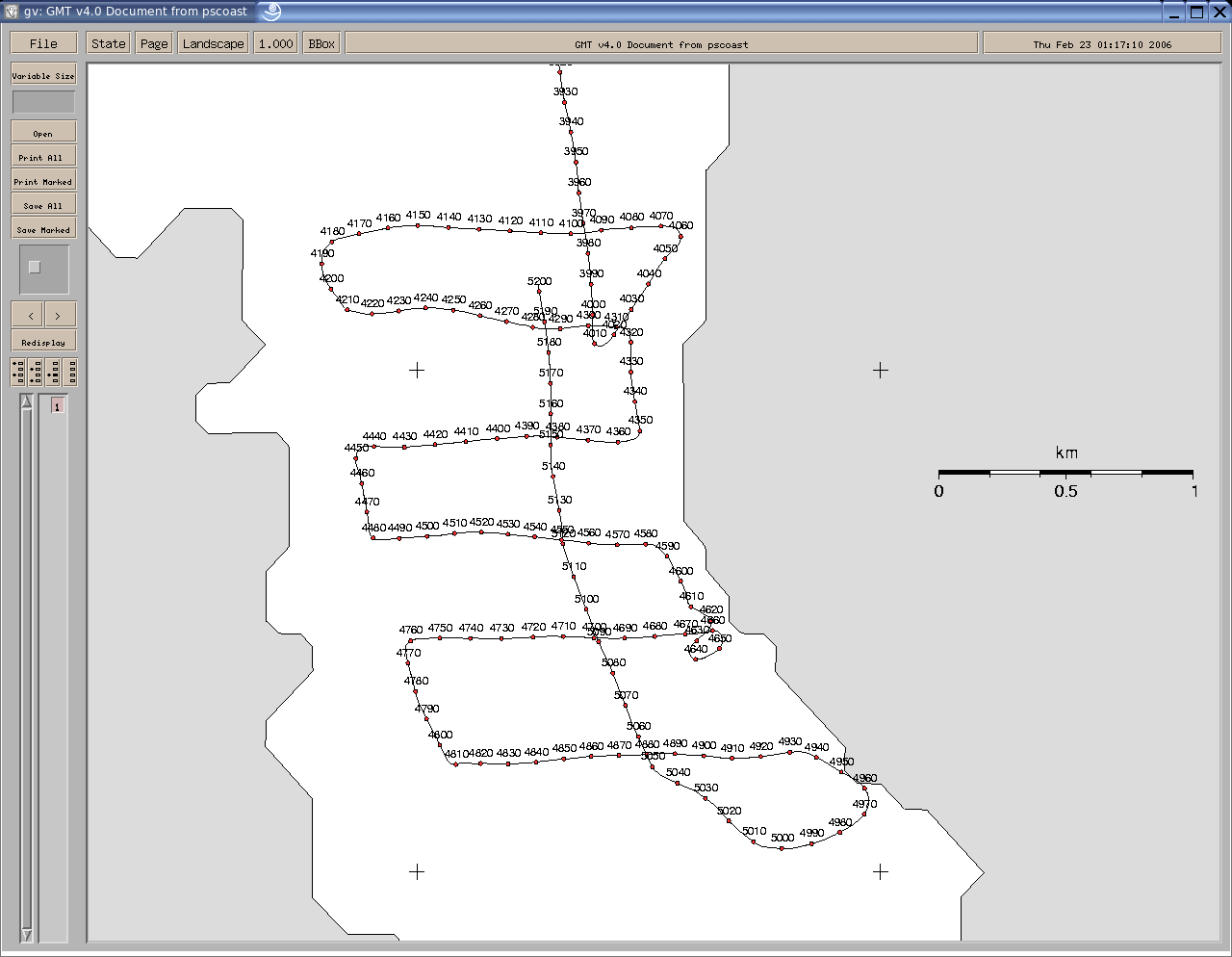
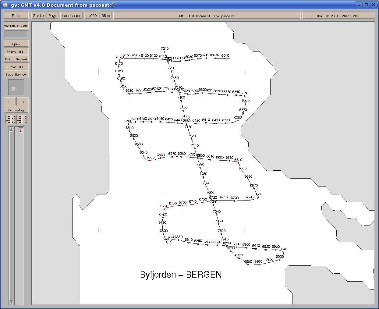
2. Shotpoint maps

Raw navigation log files converted by a script to this format - parameters are:

#SP, Date, Time hhmmss (UTC), Latitude, Longitude, Easting, Northing, UTM Zone
..
3159 14.02.2006 093536 60.512567 5.271720 295344.9 6714295.9 32V
3160 14.02.2006 093540 60.512590 5.271562 295336.4 6714298.9 32V
3161 14.02.2006 093544 60.512610 5.271402 295327.7 6714301.7 32V
..

Latitude, longitude data from Garmin GPS-35. Datum: WGS84.
Note: This is position of antenna. Offset adjustment needed to get position of streamer channel 1 midpoint.

Plotted, using Generic Mapping Tools (GMT), with this script.

Group A (click to enlarge) - PostScript.	Group A & B (click to enlarge)
Group B (click to enlarge)	Group C (click to enlarge) - PostScript

3. Seismic- & navdata

Seismic data acquisition parameters:

• 2 channels
• Sample interval: 0.125 ms (8000 Hz)
• Bandpass filter: 50 Hz - 1000 Hz

Seismic Unix used for data processing.

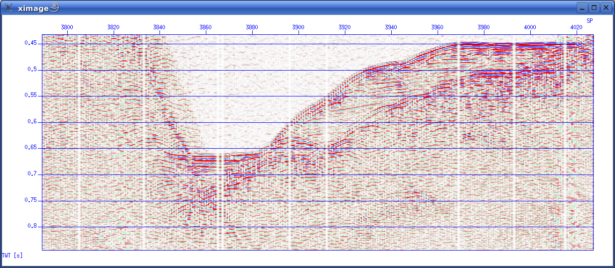
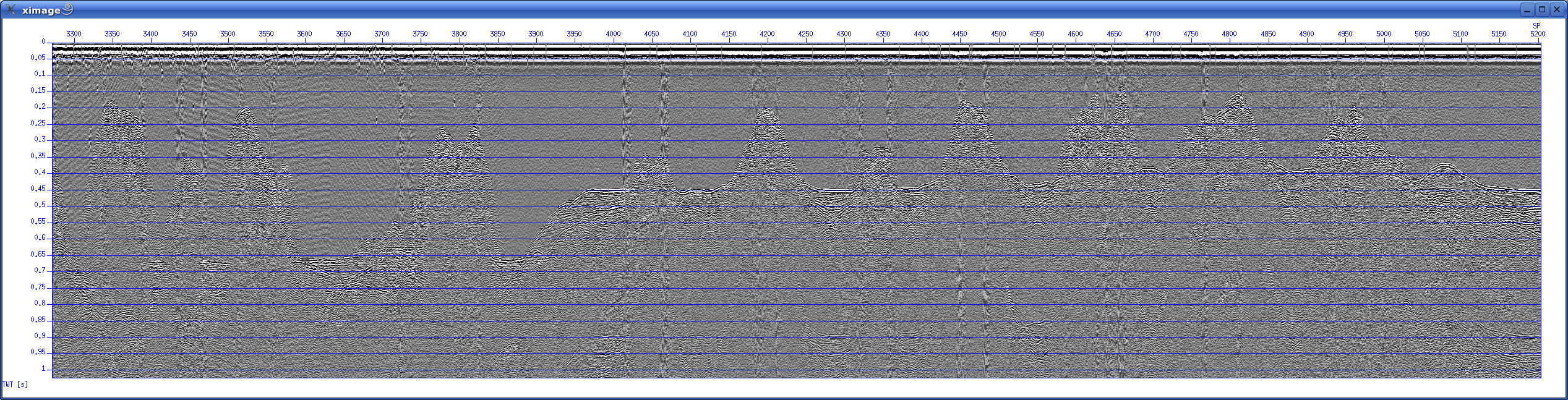
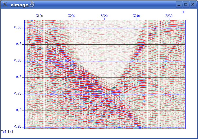
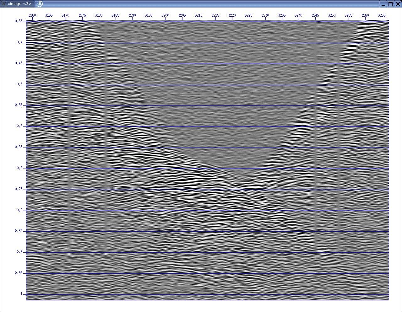
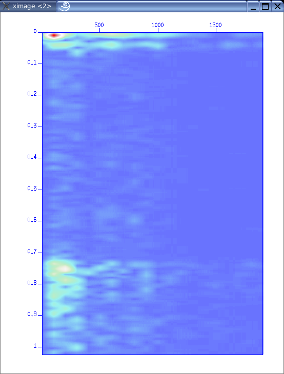
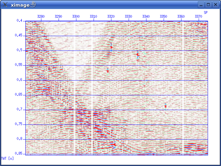
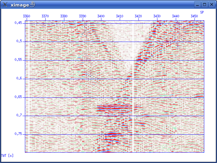
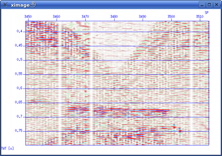
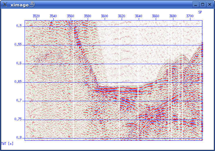
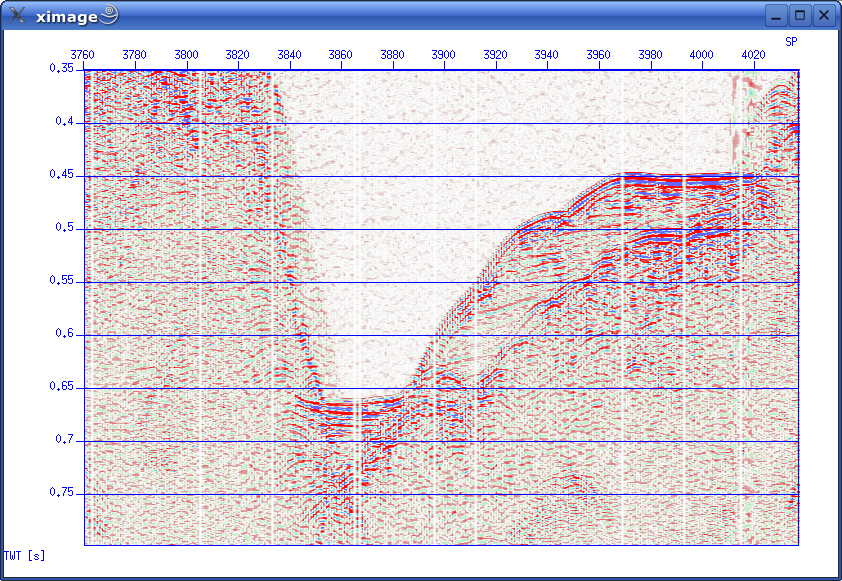
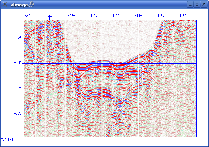
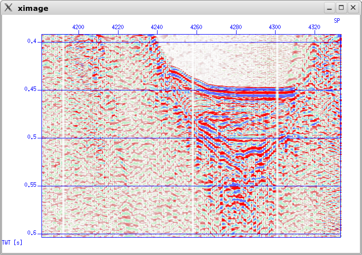
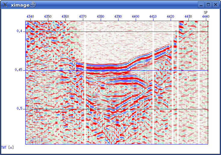
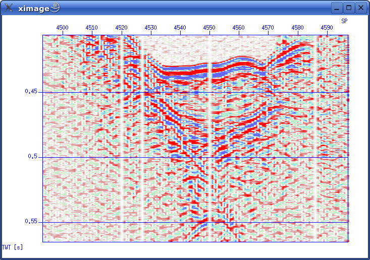
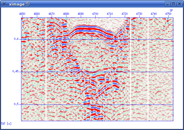
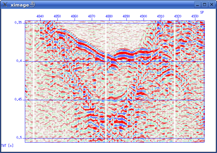
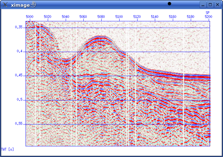
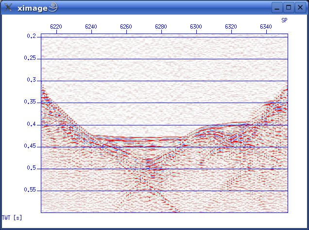
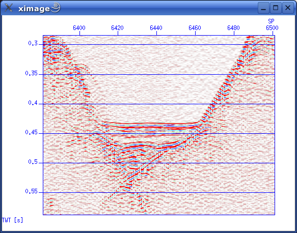
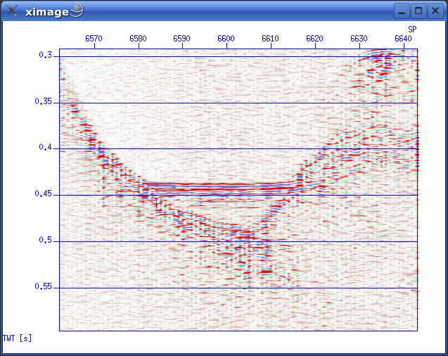
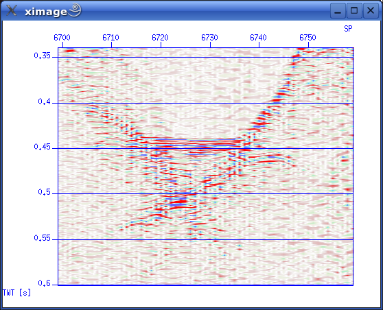
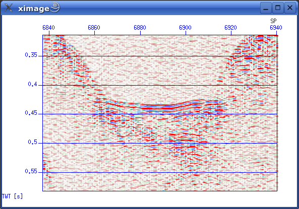
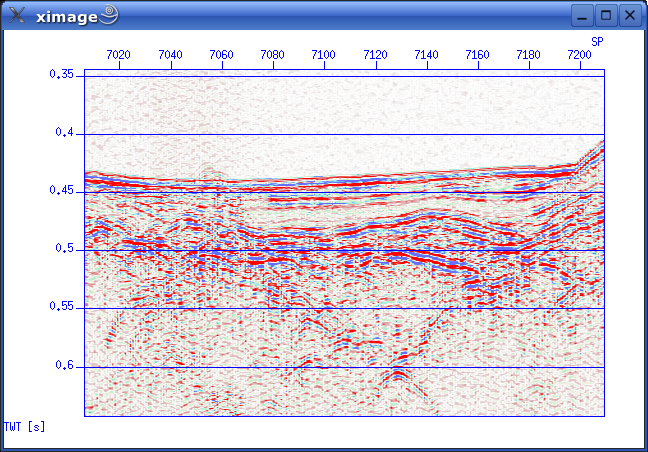
4. Seismic data previews - click to enlarge

Tilted reflectors are part of moraine from last glacialization.

Lines A2-A6 were collected as one large data file (can be split into sections, if needed)

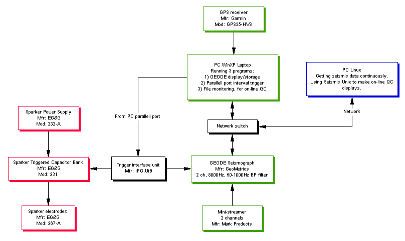
5. Instrumentation

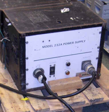
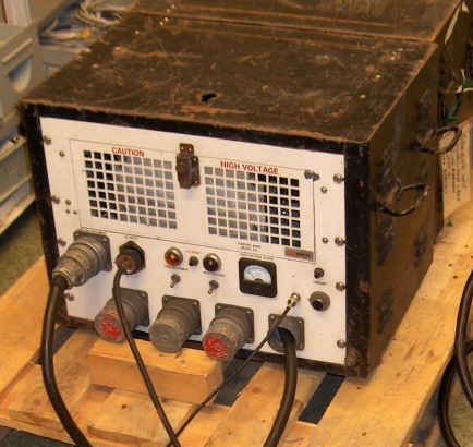
GEOL200-2006 instrumentation diagram.

Sparker source

The sparker system stores energy in a bank of high-voltage capacitors, and discharges these through the sparker electrodes in the water when the system receives a trigger pulse.

Sparker Power Supply

Sparker Triggered Capacitor Bank

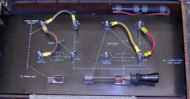
It is possible to configure the energy storage capacity by setting jumpers on the Capacitor Bank unit, as shown below:

Selecting energy storage capacity by jumper settings on the Triggered Capacitor Bank

Sparker system images: Click here.

Streamer

• Type: Two-channel mini-streamer
• Manufacturer: Mark Products Inc., Houston, USA
• Date: 7/3/1980
• Configuration:
  • Channel 1 (front): 21 ea hydrophones, 51 cm spacing
  • Channal 2: 8 hydrophones, 1.75 m spacing
• Report from latest calibration.
• Offset (distance between source and centre of first hydrophone group):
  Calculate from time between zero time and arrival of direct wave.

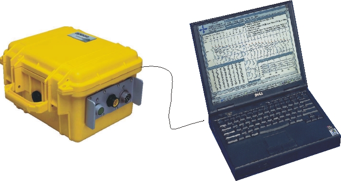
Recording

We used our excellent GEODE seismograph, manufactured by GeoMetrics. For GEODE specifications, see manufacturer's product web page.

GeoMetrics GEODE Seismograph, connected to PC laptop for display/data storage (image from manufacturer's web site).

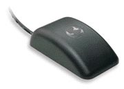
GPS Receiver

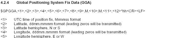
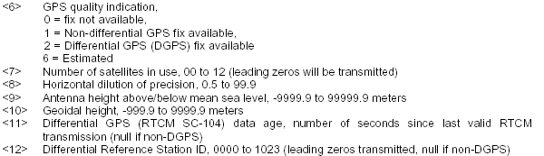
The Garmin GPS35-HVS receives GPS signals and transmits NMEA sentences via serial RS-232 interface.

Download manual from here (PDF format).

It has been configured to output the $GPGGA sentence, which has the following format (excerpt from p. 19 in the manual):

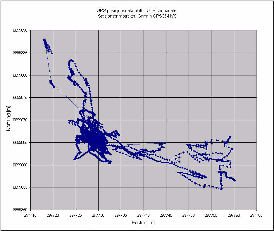
To get an idea of the GPS accuracy, here is a 3-hour position logging from a stationary GPS (click to enlarge). As you can see, the data outliers can be large. This is the reason for employing differential GPS - will use this on next RV "Hans Brattstom" survey.

3-hour positional plot from stationary GPS.

6. Software notes

Latitude / Longitude to UTM conversion.

The Garmin GPS-35 receiver can be configured to output a combination of different data telegrams, called NMEA sentences. In our case, we have selected the GPGGA sentence. The part og the GPGGA sentence that is included in the recording logfile has this format:

$GPGGA,135902,6028.5914,N,00514.8399,E,1,09,0.8

   ^     ^        ^     ^      ^     ^ ^  ^  ^
   |     |        |     |      |     | |  |  |
   |     |        |     |      |     | |  |  +----> Horizontal Dilution of precision
   |     |        |     |      |     | |  +-------> Number of satellites in view, 00 - 12
   |     |        |     |      |     | +----------> GPS Quality Indicator 0 - fix not available, 1 - GPS fix, 2 - Differential GPS fix
   |     |        |     |      |     +------------> E or W (East or West)
   |     |        |     |      +------------------> Longitude, dddmm.mmmm format (d -> degree, n -> minute)
   |     |        |     +-------------------------> N or S (North or South)
   |     |        +-------------------------------> Latitude, ddmm.mmmm format
   |     +----------------------------------------> Time (UTC)
   +----------------------------------------------> NMEA sentence ID

We wish to produce a shot event file that should have this format:

#Shotpoint, Date, Time hhmmss (UTC), Latitude, Longitude, Easting, Northing, UTM Zone
3159 14.02.2006 093536 60.512567 5.271720 295344.9 6714295.9 32V

In order to convert latitude and longitude coordinate pairs to UTM, we must first convert the (d)ddmm.mmmm to decimal degrees, i.e. (d)dd.dddddd. This is accomplished in the Decideg(t) function of this Python program.  Note the assumption made - that latitudes are north of equator, and longitudes east of the Greenwich meridian; decimal latitudes south of equator and longitudes west of Greenwich meridian are normally expressed as negative numbers.

Next step is the Latitude/Longitude to UTM conversion. Here we use a Python library called LatLongUTMconversion. The library must be downloaded and unpacked. The code can either be included in your own programs, or installed on your computer (assuming Linux, see readme file). It provides a function LLtoUTM(ReferenceEllipsoid, Lat, Long) that takes the reference ellipsoid (in our case WGS-84 = 23), and Lat/Long, in decimal degrees, as input parameters. Output is a 3-tuple consisting of UTMZone, UTMEasting and UTMNorthing.

The conversion to shotpoint file is done in line 20-23 in this program.

Reading and processing SEG-Y files from the GEODE seismograph.

Seismic data is commonly stored in SEG-Y format. We use an open-source processing package called Seismic Unix to process the seismic files. This package can be installed on any Linux box (the link provides a quick install section).

First we convert the SEG-Y file (here 3271.sgy) to Seismic Unix *.su format, using the command:

segyread tape=3271.sgy endian=0 conv=0 | segyclean > 3271.su

Use endian=0 on a little-endian CPU (like PC); conv=0 as floating-point conversion from IBM to IEEE-format is not needed in this case (see also the Data sample format code, byte # 3225 & 3226, in the SEG-Y binary header - its interpretation is described on page 6 in the SEG-Y standard, Rev 1.)

First take a look at which trace headers are in use, and their min/max range, by using the surange command:

surange < 3271.sy
3866 traces:
 fldr=(3271,5203)  tracf=(1,2)  trid=1 nvs=1 nhs=1
 scalco=1 gx=(0,1)  counit=1 ns=4096 dt=250
 lcf=50 hcf=1000 year=6 day=45 hour=(9,11)
 minute=(0,59)  sec=(0,59)  timbas=1

The streamer has two channels. We only use the first. To select data from the first channel and display these, use:

suwind key=tracf min=1 max=1 < 3271.su | suximage perc=95 key=fldr grid1=solid d1num=0.05 label1="TWT [s]" label2="SP" &

On-line QC display of data, on Linux PC

On the GEODE laptop, a Python program monitors the SEG-Y data directory and informs other units on the network that new data are available. This monitoring program is described here.

A Linux machine with Seismic Unix can receive this information and display new data in various ways. Data reception is described here. Seismic QC displays are described here.