• View
• Edit
• History
• Print

SEISMIC UNIX COURSE MAY 2007

INTRODUCTION

This course (or rather: Workshop) was arranged in May 2007 for two visitors from University of Juba, Sudan, as part of exchange arrangement between our two universities.

Department of Earth Science arranges a course in Linux/Unix scripting, Seismic Unix (seismic processing software), GMT (mapping software) and other related subjects.

Topics can be selected from list below. Course content can be tailored to suit individual participant's background and interests.

Course duration is estimated to be 2 weeks (10 days); 1-2 hours/day.

Each participant is furnished with a dual-head Linux PC where Seismic Unix and GMT are installed, in addition to all other tools that are part of a modern Linux distribution.

Ole Meyer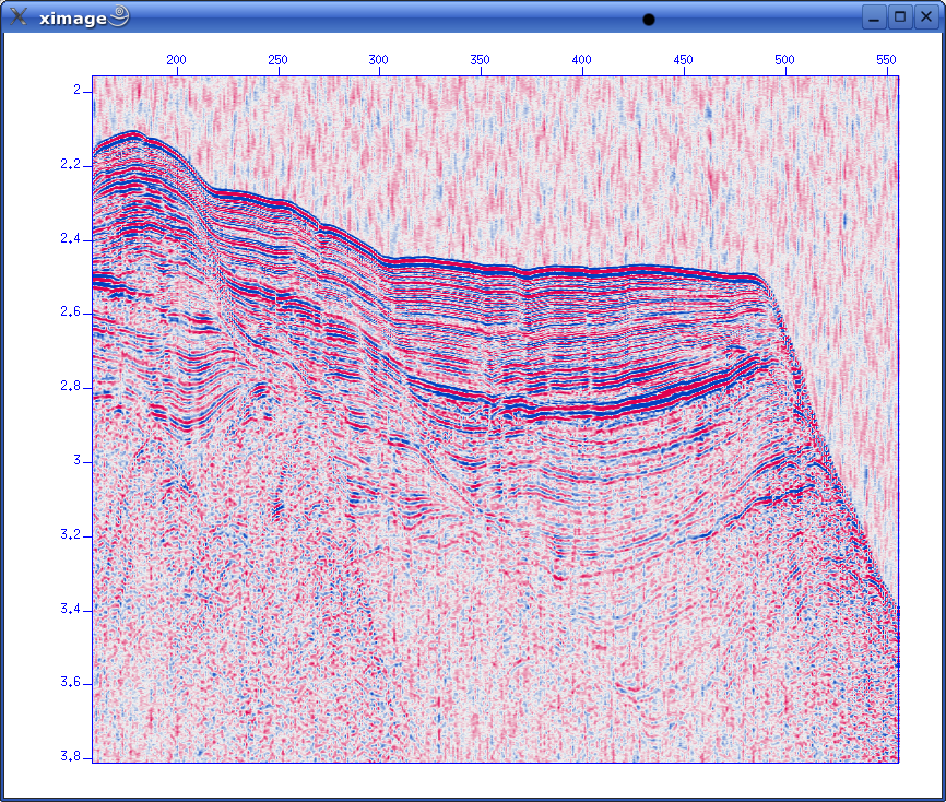
Sen. engineer
Dept. of Earth Science, University of Bergen
19 May 2007

COURSE MENU

Topics you can choose include:

Introduction to

• Linux/Unix scripting in Bash / Python.
• Seismic Unix - open Seismic processing software.
• GMT - Generic Mapping Tools - open mapping software.
• Gnuplot - open plotting software.
• Downloading and installing Linux - a hands-on example.
• Downloading and installing Wikis on a Linux server.
• Demonstration of modern seismic acquisition hardware: GEODE from Geometrics.

More details below. Please inform us on which area(s) you are most interested in. Course content can be tailored to each participant.

Linux/Unix scripting in Bash / Python

Bash

• Editor
• Making scripts executable
• Overview of most common commands
• Examples of simple scripts

Python

• A modern scripting language
• Editor
• Language overview
• Script example
• Links:
  • http://www.python.org

Seismic Unix

• The SEG-Y file standard.
• The Seismic Unix file standard, and how it differs from SEG-Y.
• Basic Seismic Unix
• Loading SEG-Y file
• Scripting Seismic Unix
• We'll use T. Benz: "Using Seismic Unix to Teach Seismic Processing".
• Links:
  • Path:./seismic-unix

GMT - Generic Mapping Tools

• What type of maps can be generated with GMT - example gallery: GMT
• A simple map - step by step
• More advanced examples

Gnuplot

• Gnuplot gallery: http://gnuplot.sourceforge.net/demo_4.5/
• A simple plot
• More advanced examples
• Links:
  • http://www.gnuplot.info

Downloading and installing Linux

We can go through the whole process, from downloading to installation, on a new PC. There are several versions of Linux (called distributions) to choose from. We are mainly using Suse here.

Downloading and installing Wikis

Wikis are very useful for group collaboration (as Wikipedia demonstrates). We'll show you how to download and install a Wiki on a Linux server.

Demo of modern seismic acquisition system

The department has a GEODE manufactured by Geometrics. We can demonstrate data collection, and also integration with GPS receivers for time and position tagging of data. Data is collected on Windows laptops; we'll transfer data to Linux PC and start processing with Seismic Unix. We will extract nav data using a small Python script, and plot these with GMT.

ONE-CHANNEL STREAMER, PART A

A single channel streamer represents one of the most simple data acquisition concepts in marine geophysics. In spite of this, it provides data of surprisingly good quality. We will use single channel streamer data as an introduction to the seismic processing software called Seismic Unix. Afterwords we will study multi-channel streamer data collected from the same survey area, so that a direct comparison is possible.

Overview

We'll take a look at line 26 from the GEOL201-2004 survey. This line (at 78 deg 15 min latitude) crosses the rift zone that runs along western part of Svalbard.

Here is an overview map of the area. The map is made with GMT and we will later see how.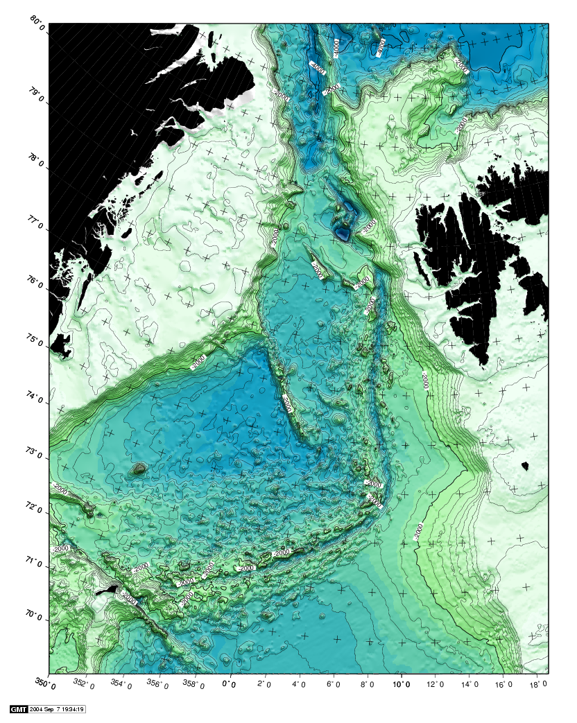

Fig.1. Overview - area between Svalbard and Greenland.

Shotpoint map line 26

Fig. 2. SP map, line 26 - click to see large version.

Get data

Make new directory

Open terminal window. Make new directory (or folder) with name ExampleA by writing mkdir ExampleA

Download

Download dataset to the newly created directory: Path:./course_S07/data/no1/line-26.su

SEG-Y file standard

You should have some basic knowledge of the SEG-Y file standard. This is provided here: SeismicUnix

Our example file is in Seismic Unix format (thus the *.su file extension). So we do not have to go through the SEG-Y import stange when we want to process the example data.

Check range of parameters in SEG-Y Trace identification headers:

In terminal window, use the SURANGE command. You should get this result:

olem@ompc3:~/www/course_S07/data/ExampleA> surange < line-26.su
1324 traces:
  tracl=(1,1324)
  tracr=(1,1324)
  fldr=(1,1324)
  tracf=1
  ns=8192
  dt=1000

This tells us that six different trace header parameters have been used:

tracl

Trace sequence number within LINE; this parameter counts traces sequentially.

tracr

Trace sequence number within reel, is our case identical to tracl.

fldr

"Original field record number" - used as shot number counter.

tracf

"Trace sequence number within original field record" - this parameter counts number of channels in the streamer. As we use a single-channel streamer, the value of tracf is constant, set to 1.

ns

Number of samples in traces.

dt

Sample interval, in microseconds.

To summarize, in this file we have 1324 traces, sample interval is 1 ms (1000 microsec.) and 8192 samples per trace. This amounts to 8.192 seconds recording time.

A first look

In terminal window use the suximage command:

suximage perc=95 < line-26.su

You should have this display: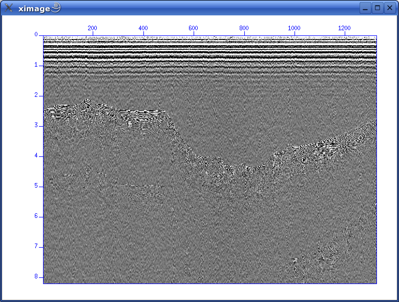

Fig. 4. First glimpse of data

Use left mouse button and zoom in on area of interest: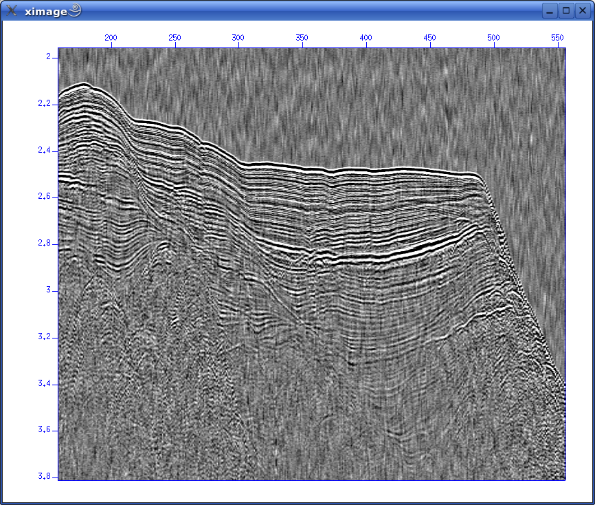

Fig. 5. Zoom in

Change colour palette by pressing "r" or "h":

Fig. 6. Change color palette by pressing "r" or "h"

Bandpass filter

Apply simple bandpass filter in the range 20 to 60 Hz:

sufilter f=10,20,60,70 < line-26.su | suximage perc=95

Here we use the important Unix (Linux) concept of piping: The output from the SUFILTER command is sent to the SUXIMAGE command. The piping symbol is the "|" sign.

We should now have this image: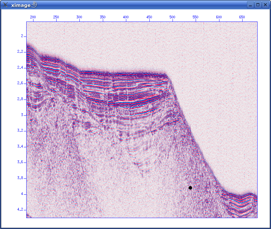

Concluding remarks

We'll continue with Seismic Unix processing Monday, at 10 a.m.

ONE-CHANNEL STREAMER, PART B

Let's reiterate what we have covered so far.

• Introduction to the SEG-Y file structure, and, in particular, the trace header parameters.
• Checking trace identification headers in a seismic data set using the SURANGE command.
• Raw display of data using the SUXIMAGE command.
• Zooming and change of color palette.
• Applying a bandpass filter using the SUFILTER command.
• Unix/Linux concept of piping - the output from one command is sent directly to another command - using the pipe symbol "|". In this way you can tie together a chain of commands.

Another Unix/Linux concept you should know: redirection

In addition to piping, Seismic Unix also relies on another Unix/Linux concept called redirection. We have already used it in the previous section.

E.g., while applying the bandpass filter, we used these commands:

sufilter f=10,20,60,70 < line-26.su | suximage perc=95

As you have probably figured out, the line-26.su is the input file to the SUFILTER command. The "<" sign takes care of this. It says that the SUFILTER command should take it's input from the file name that is provided.

In a similar fashion, the ">" sign says that the output from a command should be sent to a specified file.

Consider this example. The SUPLANE command makes a simple synthetic Seismic Unix data set. You can display the data set directly using piping, like this:

suplane | suximage

Or you can redirect the output to a file, like this:

suplane > datafile.su

Display this file:

suximage < datafile.su

Getting help with Seismic Unix commands

It's easy to get help on Seismic Unix commands. Just type the command name without any parameters: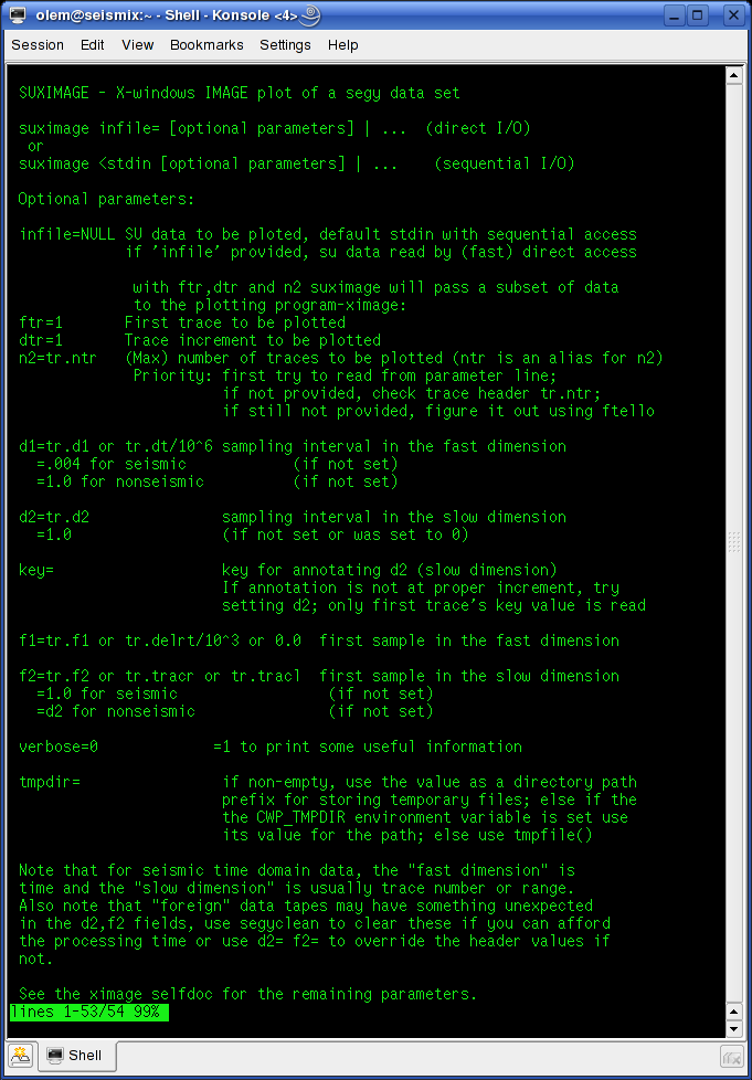

Fig. 2.1. Get help on Seismic Unix commands - just type command name without parameters.

Often one command can build on other commands. This is the case for SUXIMAGE, which is built on the XIMAGE command. So type "XIMAGE" to see details.

More Seismic Unix processing

As already mentioned, single channel streamer data represents a very simple method of geophysical data acquisition. So we don't have to do any CMP (Common Midpoint) sorting of traces, velocity analysis and stacking of data.

We will cover some common processing steps before we we continue. Please refer to section 5 of T. Benz: "Using Seismic Unix to teach seismic processing".

Data dependent amplitude corrections: AGC (Automatic Gain Correction)

Before visualizing data AGC is often applied. It means subdividing each trace into windows with a user-specified length. The RMS (root-mean-square) amplitude within the window is calculated and compared to a desired value; if these two don't match a scaling factor is applied to the samples within the window. AGC is an example of "data dependent amplitude corrections" - amplitude information from the data is used to scale it.

To apply AGC to our data set the following command is used:

sugain agc=1 < line-26.su | suximage perc=95

It will look like this: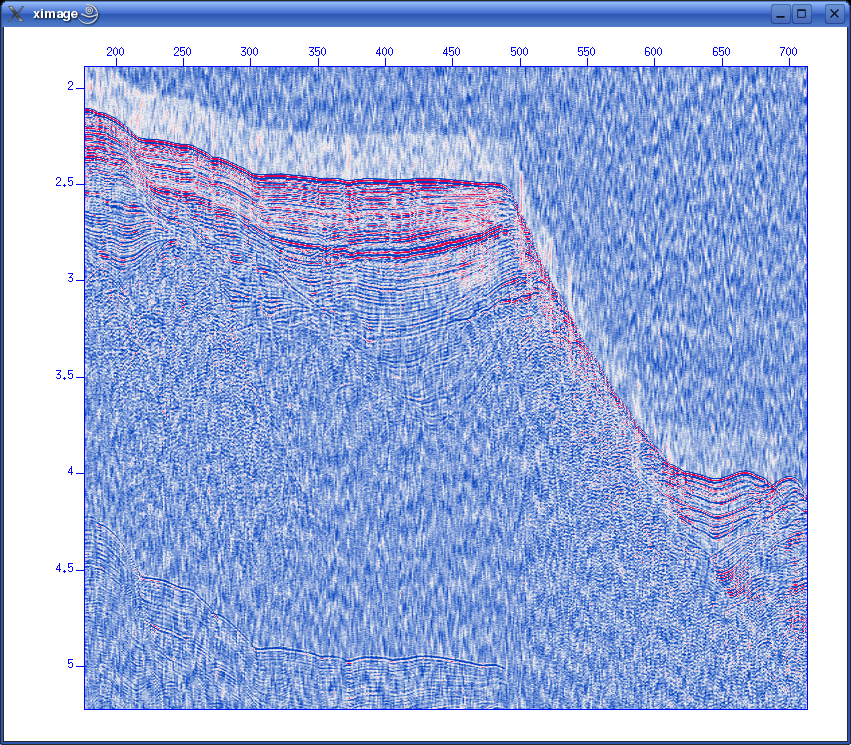

Fig. 2.2. AGC applied using default SUGAIN parameters.

Wait! What about the size of the sub-dividing windows? Isn't the user supposed to supply this piece of information?

That's correct. But the SUGAIN command will use default values if we don't supply any. To see default values, type "SUGAIN" to see all options:

SUGAIN - apply various types of gain to display traces

 sugain <stdin >stdout [optional parameters]

 Required parameters:
       none (no-op)

 Optional parameters:
       panel=0         =1 gain whole data set (vs. trace by trace)
       tpow=0.0        multiply data by t^tpow
       epow=0.0        multiply data by exp(epow*t)
       gpow=1.0        take signed gpowth power of scaled data
       agc=0           flag; 1 = do automatic gain control
       gagc=0          flag; 1 = ... with gaussian taper
       wagc=0.5        agc window in seconds (use if agc=1 or gagc=1)
       trap=none       zero any value whose magnitude exceeds trapval
       clip=none       clip any value whose magnitude exceeds clipval
       qclip=1.0       clip by quantile on absolute values on trace
       qbal=0          flag; 1 = balance traces by qclip and scale
       pbal=0          flag; 1 = balance traces by dividing by rms value
       mbal=0          flag; 1 = balance traces by subtracting the mean
       maxbal=0        flag; 1 = balance traces by subtracting the max
       scale=1.0       multiply data by overall scale factor
       norm=1.0        divide data by overall scale factor
       bias=0.0        bias data by adding an overall bias value
       jon=0           flag; 1 means tpow=2, gpow=.5, qclip=.95
       verbose=0       verbose = 1 echoes info

Possible parameters to the SUGAIN command are listed, and default values are given. In our case, we have wagc=0.5, which means that the window is 0.5 seconds long. Try experimenting with other window sizes, like:

sugain agc=1 wagc=0.25 < line-26.su | suximage perc=95

Data independent amplitude corrections: Multiplication by power of time, exponential gain

These operations don't permanently alter the data, like the data dependent operations did. If the inverse function is applied the original data can, in principle, be restored.

Using the SUGAIN command both multiplication by power of time, and exponential gain can be achieved. These two parameters must be given to the SUGAIN command:

tpow

Multiply data by t^tpow

epow

Multiply data by e^(epow*t)

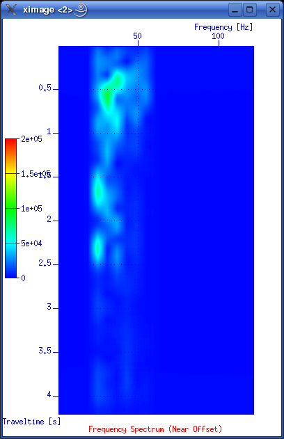
So giving this command will apply a power of time operation to data:

sugain tpow=2 < line-26.su | suximage perc=95

One parameter looks peculiar, and that is the "jon" parameter. It's actually named after one of the heavy-weights in seismic processing - Jon Claerbout, Professor at Stanford University. When you give the command

sugain jon=1 < line-26.su | suximage perc=95

your data is really exposed to SUGAIN operation with these parameter values: tpow=2, gpow=.5, qclip=.95.

Spectrum analysis - the frequency content of data

Data can be viewed in either time or frequency domain. Let's take a look at the frequency content of our data. We use the SUSPECFX command for this purpose.

suspecfx < line-26.su | suximage

This yields the following image (press "h" to obtain suitable color palette):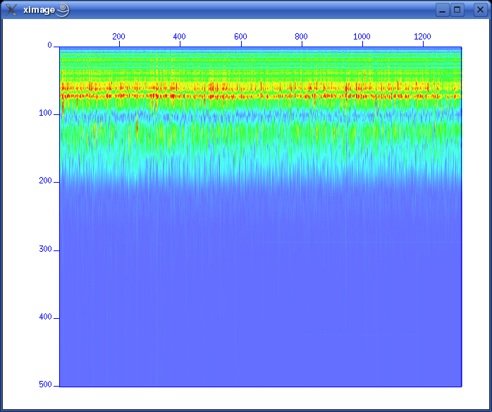

Fig. 2.4. Frequency content of data set.

Frequency is on the vertical scale, and trace number is on the horizontal.

Zooming in, we see that the energy is mainly concentrated is the frequency band between 30 and 80 Hz: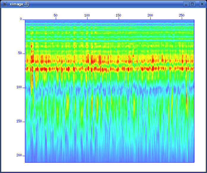

Fig. 2.5. Frequency content, zooming in.

So perhaps our choice of bandpass cutoff frequencies in previous section was not correct? Try to repeat the bandpass filter operation, but this time with 30-80 Hz range. See SUFILTER parameter description (just write "sufilter").

Selecting a single trace from the data set

Let's continue with frequency domain view of data. This time we want to look at frequency content of a single trace. So, how do we extract a single trace from the data set?

The answer is the SUWIND command.

We just have to specify which trace header parameter we wish to use as keyword in the extraction. Remember the output from the SURANGE command:

olem@seismix:~/www/course> surange < line-26.su
1324 traces:
tracl    1 1324 (1 - 1324)
tracr    1 1324 (1 - 1324)
fldr     1 1324 (1 - 1324)
tracf    1
ns       8192
dt       1000

So let's use TRACL as keyword, and extract trace number 100:

suwind key=tracl min=100 max=100 < line-26.su > tracl_100.su

Notice that we used the Unix redirect symbol ">" to save the output from the SUWIND command to a new file called tracl_100.su.

We can take a look at the so-called Gabor spectrogram of this trace. This shows instantaneous frequency content of signal as function of time:

sugabor < tracl_100.su | suximage

A plot should look like (use "h" to have suitable colors, and zoom in) this: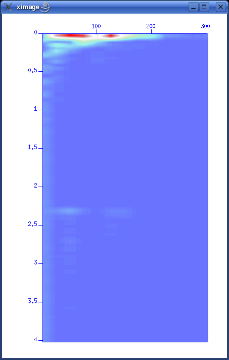

Fig. 2.6. Gabor spectrogram of trace with fldr=100.

Frequency on horizontal axis, and time on vertical. We notice how the direct source wave dominates in the beginning of the trace. After 2.3 seconds the bottom reflection shows up, as a weak replica of the source signal.

Adding annotation, grid to displays

The graphical displays we have made so far could need some improvements in terms of annotations and grid lines.

Let's use the last Gabor spectrogram as example.

sugabor < tracl_100.su | suximage title="Gabor spectrogram, fldr=100"\
label1="Time [s]" label2="Frequency [Hz]" grid1=dot grid2=dot

Note the "\" character which is used to split long commands over several lines.

Which yields: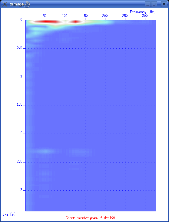

Fig. 2.6. Gabor spectrogram, fldr=100, annotation and grid lines added.

These are the options that influence display appearance. Write XIMAGE and scroll down ...: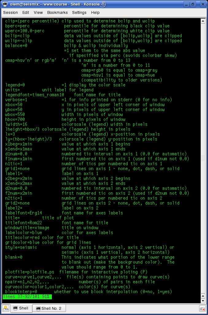

Fig. 2.7. Part of XIMAGE option description; parameters that influence annotation and grid lines.

Problems ahead

The last command was rather lengthy. If we were to write this command each time, possibly as part of a chain of commands, we would soon run out of patience. The solution is scripting. This will become a topic in start of the next section.

SCRIPTING

Instead of typing commands in terminal window we collect all commands in file that can be executed. These files are called scripts.

All commands available in a terminal window represents a particular shell language. It's important to be aware of the existence of several different shell languages in the Unix/Linux world. They share some common traits, but there are also differences that can cause problems for beginners.

The default shell language used in most Linux distributions is called Bash.

Scripts are written with editors. Emacs and vi are common Unix household editor names; however they are a bit old-fashioned and beginners should opt for more modern versions. Here we will use an editor called kate, so open a new terminal window and type "kate".

There are many different Unix/Linux shell languages - Bash, tsh, csh .. Here are some introductory Bash links: http://pegasus.rutgers.edu/~elflord/unix/bash-tute.html http://tiger.la.asu.edu/bash_tutorial.htm http://tille.garrels.be/training/bash/index.html

First kate session

Copy & paste the following text into the new empty kate file:

#!/bin/bash

# The "#" symbol starts comments lines
# The first line in script is special - it invokes the shell interpreter

sugabor < tracl_100.su | \
   suximage title="Gabor spectrogram, fldr=100" \
            label1="Time [s]" label2="Frequency [Hz]" grid1=dot grid2=dot \
            windowtitle="Seismic Unix scripting is fun!" \
            gridcolor=white \
            titlecolor=black \
            labelcolor=black \
            wbox=800 \
            hbox=900 \
            cmap=hsv4

# Due to the line continuation character ("\") the above lines will be
# treated as a single line.

# NOTE: The script must be made executable, by writing "chmod +x [script name]"

Save the file as script1.sh into the folder where the seismic data is placed.

The editor should now look like this: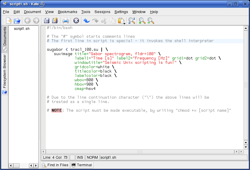

Fig. 3.1. First kate session.

Open terminal window, cd to script folder, and make it executable by typing "chmod +x script1.sh".

Execute the file by typing "./script1.sh".

Hopefully your first script result pops up. We have used the same SUGABOR command as in last example of section 2 - with the addition of some new SUXIMAGE options (type "ximage" to see option description).

Exercise Alter range of axis so that frequency is within 0 - 250 Hz, and time within 0 - 4 seconds.

Using script from T. Benz: "Using Seismic Unix to teach ..."

We'll continue with a script from T. Benz: "Using Seismic Unix to teach ...", chapter 5, page 69, called filt.scr.

This script is a bit more advanced.

Copy this section to a new empty file in kate:

#! /bin/sh

echo "Bandpass Filter Test" 

indata=ozdata.25.sw
rm -f tmp*
tpow=2.0

#------------------------------------------------
# Show the original Shotplot and Spectrum first..
#------------------------------------------------

sugain <$indata tpow=$tpow >tmp0 

suxwigb <tmp0 perc=90 xbox=10 ybox=10 wbox=400 hbox=600 \
        label1="Traveltime [s]" label2="Offset [m]"\
        title="Original Shot Gather" verbose=0 key=offset &

suwind <tmp0 key=offset min=-50 max=50 |
sustack key=dt | 
sugabor fmax=125 band=6 |
suximage xbox=420 ybox=10 wbox=400 hbox=600 bclip=2e05 wclip=0 \
         label1="Traveltime [s]" label2="Frequency [Hz]" \
         title="Frequency Spectrum (Near Offset)" \
         grid1=dot grid2=dot cmap=hsv2 legend=1 \
         verbose=0 &

#------------------------------------------------
# Bandpass Filter Test...
#------------------------------------------------

ok=false
while [ $ok = false ]
do
  rm -f tmp1
  if [ $selection ]
  then
    echo "Bandpass Filter Test"
    echo "Press A to add a filter"
    echo "Press S to start over"
    >/dev/tty
    read choice1
      case $choice1 in
      [sS]) cp tmp0 tmp1
            echo "-> Using original data";;
      [aA]) cp tmp2 tmp1
            echo "-> Using filtered data";;
      esac
  else
    cp tmp0 tmp1
  fi
  echo "Select a filterband [Hz]:"
  echo "Input: a,b,c,d  -  a:=lowcut    b:=lowpass"
  echo "                   c:=highpass  d:=highcut"
  >/dev/tty 
  read band
  sufilter <tmp1 f=$band amps=0,1,1,0 >tmp2

#------------------------------------------------
# Plot the filtered data...
#------------------------------------------------

  suxwigb <tmp2 xbox=10 ybox=10 wbox=400 hbox=600 \
          label1="Traveltime [s]" label2="Offset [m]"\
          title="Filtered Data" verbose=0 perc=90 \
          key=offset &

  suwind <tmp2 key=offset min=-50 max=50 |
  sustack key=dt | 
  sugabor fmax=125 band=6 |
  suximage xbox=420 ybox=10 wbox=400 hbox=600 \
           labeil1="Traveltime [s]" label2="Frequency [Hz]" \
           title="Frequency Spectrum (Near Offset)" \
           grid1=dot grid2=dot legend=1 bclip=2e05 wclip=0 \
           cmap=hsv2 verbose=0 &

  sufilter <tmp2 f=$band amps=1,0,0,1 |
  suxwigb  xbox=830 ybox=10 wbox=400 hbox=600 perc=90\
           label1="Traveltime [s]" label2="Offset [m]"\
           title="Rejected Data" verbose=0 perc=90 \
           key=offset &

#------------------------------------------------
# Go back or exit...
#------------------------------------------------

  echo "Press 1 for more filter testing"
  echo "Press 2 for PS output of current file and EXIT"
  >/dev/tty
  read selection
    case $selection in
	1) clear
           ok=false;;
	2) pause exit
	   ok=true;;
     esac
  done

rm -f tmp*

exit

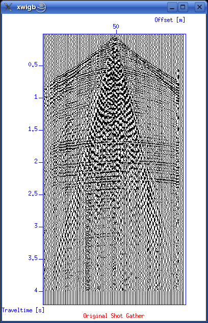
You can also download script file (right-click link and save in data directory: Path:./course_S07/data/no3/filt.scr

Then download example seismic file used (right-click and save in data directory: Path:./course_S07/data/no3/ozdata.25.sw

Make script executable by writing "chmod +x filt.scr".

Execute script by typing "./filt.scr".

Two graphical windows should appear:

Fig. 3.2. Original data

Fig. 3.3. Gabor spectrogram of original data (stacked traces near-offset)

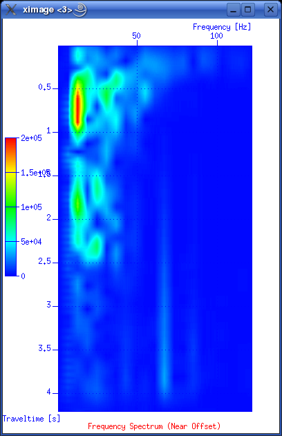
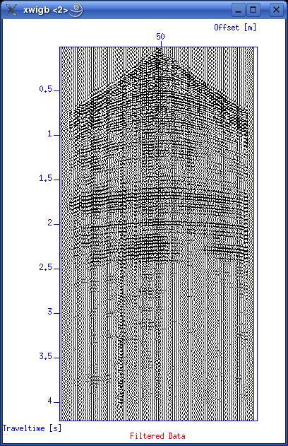
Now you can change filter parameters interactively. Let's try to get rid of low-frequency direct arrivals which appears as a reverse V-shape. From frequency spectrum we notice the high energy section below 20 Hz, so we can try a bandpass filter in the range 20 - 60 Hz. So type "20,25,60,70" in xterminal window, and press <ENTER>. Now these three new windows will appear:

Fig. 3.4. Bandpass filtered data.	Fig. 3.5. Rejected data (see below).
Fig. 3.6. Gabor spectrogram of filtered data.

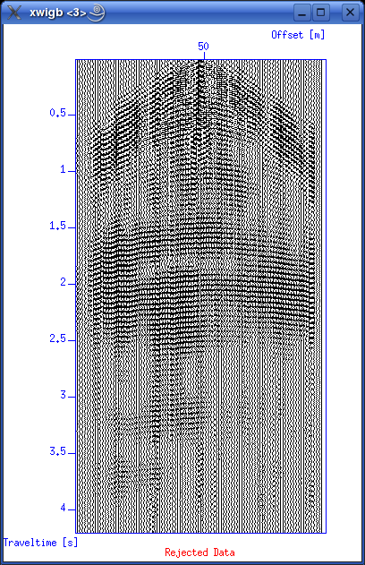
Compare the two frequency spectrums. Notice how the sub-20Hz sections is subdued by the filter applied. Also notice the display of rejected data in fig 3.5 - how is this accomplished in the script? The answer lies in this section (below "Plot the filtered data..." heading):

  sufilter <tmp2 f=$band amps=1,0,0,1 |
  suxwigb  xbox=830 ybox=10 wbox=400 hbox=600 perc=90\
           label1="Traveltime [s]" label2="Offset [m]"\
           title="Rejected Data" verbose=0 perc=90 \
           key=offset &

SUFILTER has a parameter called amps=1,0,0,1, which makes a BAND-STOP filter instead of a BAND-PASS. The f=$band means that the values we entered from the keyboard -"20,25,60,70" - are transferred, via a shell script variable called band, to the f-parameter.

We have introduced a new - perhaps the most common - way of plotting seismic data - WIGGLE PLOTS - see fig. 3.2, 3.4 and 3.5. This is accomplished by the SUXWIGB command.

IMPORTING SEG-Y DATA

We've so far looked at some basic Seismic Unix commands for plotting and processing. We'll now try to access a public domain SEG-Y dataset, unpack it, import in into Seismic Unix and display raw data.

Accessing public domain SEG-Y datasets

There are several sources of public domain SEG-Y seismic datasets on the internet. We will access data from the Marine Seismic Data Center at University of Texas, Austin: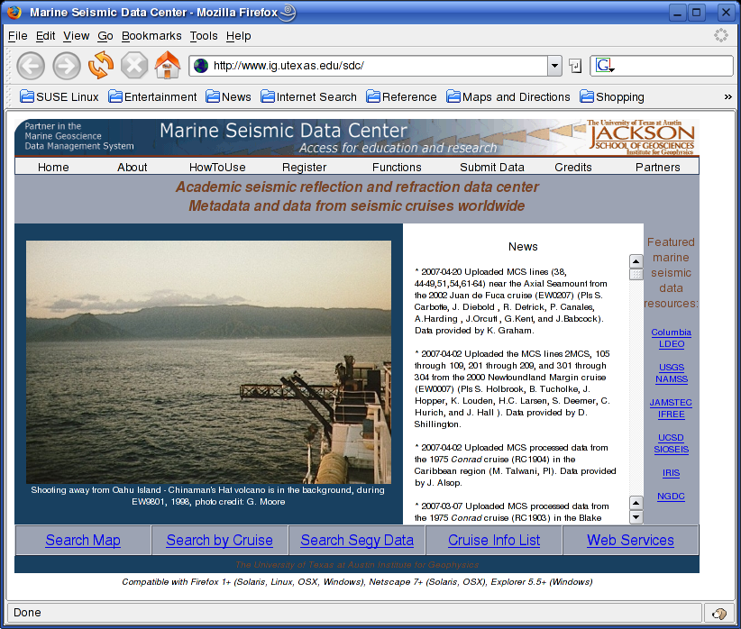

Fig. 4.1. Marine Seismic Data Center at University of Texas web page.

You first have to register to download data. After that you can browse their repository of seismic datasets and select items for downloading. Some data sets have restricted access, but many are free to download. It's important to credit the Marine Seismic Data Center in any use of their data.

We will use a data set from the Moroccan Margin. The complete citation is as follows:

After marking data sets for download, and also specifying desired file compression type, you receive a mail with download instructions. In our case we use *.tar.gz file compression format, which is very common in the Unix/Linux world - similar to the ZIP format used on Windows machines. 'tar' means that several files have been assembled into one file (called a tar file), using the Unix tar command. The gz extension means that the tar file has undergone a compression with the Unix gzip utility.

First make new directory called "no4" and cd to this directory: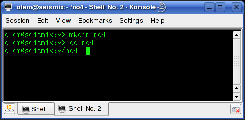

Download the file - right click and save as - to the no4 directory:

Path:./course_S07/data/no4/segy-sample.tar.gz

Unpack the file by typing:

tar -xzvf segy-sample.tar.gz

If you list the content of no4 directory you will find that three new sub-directories have been created by the unpacking command; they are called Citations, DBseis and DBtar. In the Citations you fin the citation text as rendered above. The seismic data is in DBseis -> rc2405. The seismic file is called ar54.5126.rc2405.364a.stack.segy

We are now ready to import this data set.

Importing SEG-Y data

First cd to the directory that contains the seismic file ar54.5126.rc2405.364a.stack.segy.

Import file to Seismic Unix format by typing:

segyread endian=0 conv=1 tape=ar54.5126.rc2405.364a.stack.segy | segyclean > moroccan_margin.su

There are some important issues we must treat in detail. Without knowledge of these you are bound to run into trouble later on.

Big- or little-endian?

Big- or little-endian refers to two alternative ways of storing or transmitting multi-byte data - like integers. The two methods are dependent on choice of computer CPU (Central Processing Unit) architecture.

Quoting from Wikipedia article on "Endianness":

Ordinary PCs, powered by Intel or AMD CPUs, are little-endian. Many Unix workstations use Sun or Motorola CPUs, which are nomally big-endian.

When importing SEG-Y data there is a parameter that specify the type of machine you are using. In our case - using Intel-based PCs - we have to specify endian=0.

Floating-point format: IBM or IEEE-754?

Samples in SEG-Y files are normally stored as floating-point numbers. In the first issue of the SEG-Y standard (1975), the floating point format was set to adhere to the so-called IBM standard. The problem is that modern computers use a slightly different floating point format called IEEE-754.

When importing SEG-Y data we must use an option called conv to specify whether conversion from IBM format to IEEE-754 will take place or not.

See documentation by typing segyread.

A mistake in big- or little-endianness is easy to detect. Seismic Unix will not be able to make any sense of a file with the wrong endian format. Mixing up floating point formats are much easier and may pass undetected. See this article (PDF): SEG-Y Floating Point Confusion

Checking and plotting data

Let's check trace header parameters used and their range:

olem@seismix:~/www/course/no4/DBseis/rc2405> surange < moroccan_margin.su
7129 traces:
tracr    1 7129 (1 - 7129)
fldr     1114 8402 (1114 - 8402)
tracf    1 11 (1 - 1)
cdp      1114 8402 (1114 - 8402)
cdpt     1
trid     1
nhs      1 58 (27 - 46)
duse     1
scalco   -1000
sx       -59569569 0 (0 - -45848088)
sy       0 111144737 (0 - 110962670)
counit   2
delrt    1000 5000 (5000 - 2000)
ns       1535
dt       8000
year     1983
day      120 122 (120 - 122)
hour     0 23 (17 - 8)
minute   0 59 (26 - 51)
sec      4 48 (8 - 44)

And plotting:

suximage perc=95 < moroccan_margin.su

which results in (zoom, change colour palette by pressing "r"):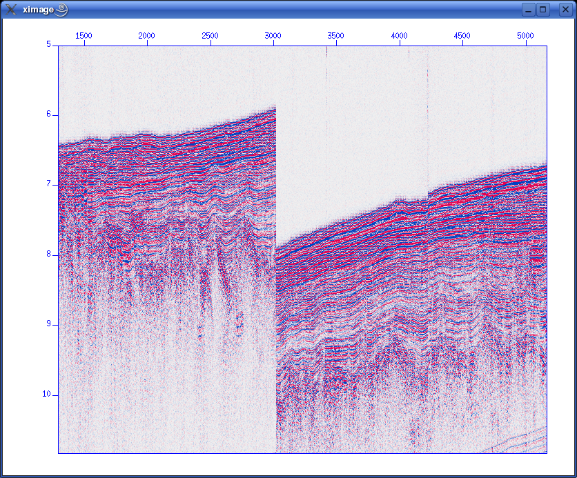

Oops. There is a problem with this file. To reduce file size the water column has been removed in various stages. We need to have all traces refer to a common start point in time.

The SUSHIFT command can fix this. If we type:

sushift tmin=0.0 tmax=15.0 < moroccan_margin.su > moroccan_margin.su.sushift

we will get what we want: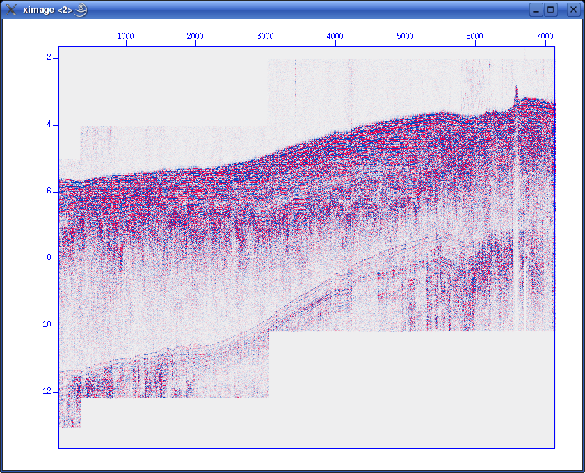

Format information present in SEG-Y binary header

The SEG-Y has a 3600-byte Reel identification header that consists of a EBCDIC Card Image Header of 3200 bytes, and a Binary Header of 400 bytes. Within the Binary Header there is a parameter located in byte no. 25 & 26 that describes the sample format used. Here are the alternatives:

 Data sample format code:                                          
   1 = 32-bit IBM floating point                                 
   2 = 32-bit fixed-point (integer)                              
   3 = 16-bit fixed-point (integer)                              
   4 = 32-bit fixed-point with gain code (integer)               
   5 = 32-bit IEEE floating point                                
   6,7 = Not currently used                                      
   8 = 8-bit, two's complement integer  

Notice that you will normally see format code 1, 32-bit IBM floating point. The 2002 revision of the SEG-Y standard introduced a new format, no. 5, which uses the modern floating point format (IEEE). Newer SEG-Y files might use this floating point standard. In that case, you should not attempt to do any floating point conversion, so the conv option to SEGYREAD should be set to zero. BEWARE: Default value is conv=1 - so there will be a conversion if you omit or forget the conv flag.

The BHEDTOPAR Seismic Unix command allows you to inspect the content of the binary header, including the parameter that describes the floating point format. When importing a SEG-Y file with SEGYREAD, both the EBCDIC and binary file header will be placed in two files with default names binary and header. In our example file from the Moroccan Margin, we have this content of the binary header:

olem@seismix:~/www/course/no4/DBseis/rc2405> bhedtopar < binary output=binary.par
jobid=0
lino=364
reno=0
ntrpr=0
nart=0
hdt=8000
dto=8000
hns=1535
nso=0
format=1
fold=0
tsort=4
vscode=0
hsfs=0
hsfe=0
hslen=0
hstyp=0
schn=0
hstas=0
hstae=0
htatyp=0
hcorr=0
bgrcv=0
rcvm=0
mfeet=1
polyt=0
vpol=0

The format is 1 (IBM floating point), as expected.

Download the SEG-Y standard from the SEG website: http://seg.org/publications/tech-stand/ Here you will also find the standard used for exchange of navigational data - UKOOA P1/90 - which we will study in the next section.

NAVIGATION DATA

Navigation data can either be included in SEG-Y data file, or available as separate file. In the latter case, often the UKOOA P1/1990 format is used. We will look into both cases.

Navigation data as part of SEG-Y file

Coordinate parameters in 240-byte trace header

In the SEG-Y file standard there are trace header parameters for both SOURCE and RECEIVER locatation. In addition there are parameters that describe coordinate format and scaling factor, if any. All these parameters are located as follows:

----------------------------------------------------------------------------------------
Byte #    2/4-byte   SU Keyword    Description                                                          
----------------------------------------------------------------------------------------
071 - 072    2       scalco        Scalar for coordinates (+ = multiplier, - = divisor).                
073 - 076    4       sx            X source coordinate.                                                 
077 - 080    4       sy            Y source coordinate.                                                 
081 - 084    4       gx            X receiver group coordinate.                                         
085 - 088    4       gy            Y receiver group coordinate.                                         
089 - 090    2       counit        Coordinate units (1 = length in meters or feet, 2 = arc seconds).  

Byte # refers to position within 240-byte trace header.

If the SEG-Y file contains shot gathers, i.e. unstacked data, both SOURCE and RECEIVER locations can be included. If the SEG-Y file contains stacked data they are normally sorted by CMP (Common Midpoint) and location coordinates refer to CMP positions. Either SOURCE or RECEIVER parameters can be used for CMP posistions (there does not seem to be a convention regarding this).

The SCALAR parameter is self-explanatory.

COORDINATE UNITS are either 1 = length in meters or feet, or 2 = arc seconds. In either case additional information about map datum is needed to obtain unambigous location information. This is often stated in the EBCDIC file header.

Navigation data in Moroccan Margin data set.

Let's recall the SURANGE information we got from the Maroccan Margin dataset. We must use the SUSHIFTED file, like this:

olem@seismix:~/www/course/no4/DBseis/rc2405> surange < moroccan_margin.su.sushift
7129 traces:
tracr    1 7129 (1 - 7129)
fldr     1114 8402 (1114 - 8402)
tracf    1 11 (1 - 1)
cdp      1114 8402 (1114 - 8402)
cdpt     1
trid     1
nhs      1 58 (27 - 46)
duse     1
scalco   -1000
sx       -59569569 0 (0 - -45848088)
sy       0 111144737 (0 - 110962670)
counit   2
ns       1875
dt       8000
year     1983
day      120 122 (120 - 122)
hour     0 23 (17 - 8)
minute   0 59 (26 - 51)
sec      4 48 (8 - 44)

We notice that counit = 2, which means that coordinates are given in arc seconds. Also, the scaling factor is -1000, meaning division by 1000.

The data repository at Texas University also provides a survey map: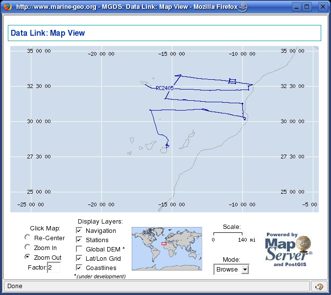

Fig. 5.1. Survey map, example data

The SEG-Y file we use contains data from start of survey - the first segment going in the west-east direction.

We now need to extract coordinates from the SEG-Y file. We use the SUGETHW (Get Header Words) command and store coordinate data to a text file we call moroccan_margin.navdata.txt:

sugethw < moroccan_margin.su.sushift key=cdp,sx,sy output=geom > moroccan_margin.navdata.txt 

Opening this txt file in kate we see:

1114 0 0 
1115 0 0 
1116 0 0 
1117 0 0 
1118 0 0 
1119 0 0 
1121 -59569569 110820762 
1122 -59567684 110820784 
1123 -59565799 110820806 
1124 -59563914 110820828 
1125 -59562029 110820850 
1126 -59560144 110820872 
1127 -59558259 110820894 
1128 -59556374 110820916
... 

We have three coloums: CMP number, sx, and sy. The first six lines do not contain location data, so we can just cut these lines and save the file again.

We have now extracted navigation data from the SEG-Y data set.

Converting arcseconds to decimal degrees

To prepare data for plotting, arcsecond navigation coordinates must be converted to decimal degrees. But how?

We have four ways to accomplish the conversion:

1. Importing data to spreadsheet program and doing the calculations there.
2. Using Bash shell language
3. Using awk, a very versatile Unix/Linux utility
4. Using a modern scripting language, like Python

Let's try Python. Copy this script to a new file in the kate editor.

#! /usr/bin/python

'''Conversion of arcseconds to decimal degrees.
Assuming input file has these data columns:  cmp, x, y
University of Bergen
Dept. of Earth Science
O.M. 24 May 2007
'''

from string import split
import sys

FileName = sys.argv[1]  # Get filename to process

f = open(FileName)

# Loop over all lines in input file. Extract cmp, x, y.
# Devide x,y by 1000, convert to decimal degrees.
# Write to output.

for line in f:
	s	= line.split()
	cdp = s[0]
	x   = float(s[1])   # First extract from line
	y   = float(s[2])

	x = x/1000          # First apply scale factor "-1000"; meaning division by 1000
	y = y/1000

	x = x/3600          # Convert from arcseconds to decimal degrees
	y = y/3600

	print cdp, x, y

f.close()

Save file with name arcseconds-to-decimal-degrees.py. Make script executable by typing

chmod +x arcseconds-to-decimal-degrees.py

Execute script, assuming you saved in in the directory where the extracted navigation data are:

./arcseconds-to-decimal-degrees.py moroccan_margin.navdata.txt

The screen output should be: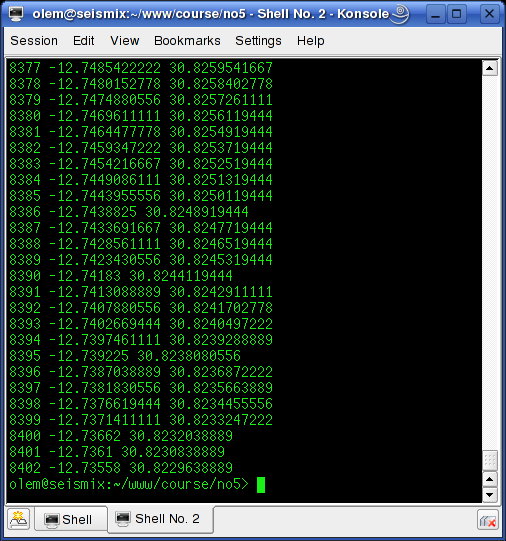

Save to file instead:

./arcseconds-to-decimal-degrees.py moroccan_margin.navdata.txt > moroccan_margin.navdata.decimal.txt

The UKOOA P1/1990 navigation file format

The UKOOA P1/90 format specification can be downloaded from SEG website. It's a fixed-position format without any <SPACE> or <TAB> separators between fields, so it can be hard to read. However, by inserting appropriate comment field in the header, it can be made much more legible, as this example shows:

H0100 SURVEY AREA ISFJORDEN, SVALBARD
H0101 SURVEY DETAILS SVALEX-2005
H0102 VESSEL DETAILS R.V. HAAKON MOSBY
H0104 STREAMER DETAILS 240 CH GECO NESSIE-3
H0200 SURVEY DATE AUGUST - SEPTEMBER 2005
H0201 FILE CREATED 16-Jan-2006
H0202 FILE VERSION UKOOA P1/1990
H0300 CLIENT SVALEX-2005
H0400 GEOPHYSICAL CONTRACTOR UNIVERSITY OF BERGEN, NORWAY
H0500 POSITIONING CONTRACTOR N/A
H0600 POSITIONING PROCESSING O.M. UNIVERSITY OF BERGEN, DEPT OF EARTH SCIENCE
H0700 POSITIONING SYSTEM
H0700 SURVEY COMPUTER SOFTWARE NAVIPAC, EIVA, DENMARK
H0700
H0800 SHOTPOINT POSITION CENTRE OF SOURCE
H1000 CLOCK TIME UTC
H0900 OFFSET SHIP SYSTEM TO SP 70.0 M BEHIND
H1200 SPHEROID AS SURVEYED A,1/F WGS-84 Spheroid 6378137.000 298.2572236
H1300 SPHEROID AS PLOTTED A,1/F WGS-84 Spheroid 6378137.000 298.2572236
H1400 GEODETIC DATUM AS SURVEYED WGS-84
H1500 GEODETIC DATUM AS PLOTTED WGS-84
H1700 VERTICAL DATUM SL : ECHO SOUNDER
H1800 PROJECTION 001 UTM NORTHERN HEMISPHERE
H1900 ZONE 33X NORTHERN HEMISPHERE
H2000 GRID UNIT 1 METRE
H2001 HEIGHT UNIT 1 METRE
H2002 ANGULAR UNITS 1 DEGREES
H2200 CENTRAL MERIDIAN 15 DEG E
H2600
H2600 00011111111112222222222333333333344444444445555555555666666666677777777778
H2600 78901234567890123456789012345678901234567890123456789012345678901234567890
H2600 -NAME-><->---<-SP-><---LAT--><--LONG---><--EAST-><-NORTH-><-DEP><D><TIME>-
SLine34-05             18781022.23N 141348.31E 482384.58677774.7 215.8242180734
SLine34-05             19781023.47N 141353.32E 482416.98677812.8 214.7242180755
SLine34-05             20781024.73N 141358.24E 482448.78677851.4 212.3242180816
SLine34-05             21781026.00N 1414 3.08E 482480.08677890.4 209.6242180837
SLine34-05             22781027.28N 1414 7.88E 482510.98677929.7 207.6242180858
SLine34-05             23781028.53N 141412.83E 482543.08677968.1 206.2242180919
...

The lines starting with H2600 are just comments. You will notice that:

Degrees (D), Minutes (M) and Seconds (S) of Latitude/longitude as given as (D)DDMMSS.SS. Notice the longitudes marked like this: 1414 3.08E. Here we have 3.08 seconds, and the leftmost field is simply vacant; the same applies to the Minute and Degree fields, should they only need one digit.

GENERATING SYNTHETIC DATA

Course participants expressed a wish to continue with Seismic Unix for the rest of the course. So GMT will have to wait for another occasion.

We will generate a synthetic dataset built on T.Benz layered earth model shown below.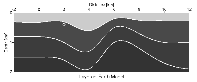

Fig. 6.1. Layered earth model, from T. Benz "Using Seismic Unix to Teach Seismic Processing".

Using 60 "geophones" we will shoot a survey over this model, and then process data. This sections details the earth model and the data acquisition process.

Layered earth model.

The earth model is generated by the following script. Copy & paste to new kate editor window

#! /bin/sh

datafile=model.data

trimodel xmin=-2 zmin=0 xmax=12.0 zmax=2.0 \
         1 xedge=-2,0,2,4,6,8,10,12 \
           zedge=0,0,0,0,0,0,0,0 \
           sedge=0,0,0,0,0,0,0,0 \
         2 xedge=-2,0,2,4,6,8,10,12 \
           zedge=0.3,0.32,0.3,0.6,0.2,0.25,0.25,0.25 \
           sedge=0,0,0,0,0,0,0,0 \
         3 xedge=-2,0,2,4,6,8,10,12 \
           zedge=0.8,0.8,1.0,1.3,0.5,0.7,1.0,1.0  \
           sedge=0,0,0,0,0,0,0,0 \
         4 xedge=-2,0,2,4,6,8,10,12 \
           zedge=1.5,1.5,1.6,1.9,1.0,1.2,1.7,1.9 \
           sedge=0,0,0,0,0,0,0,0 \
         5 xedge=1.9,2.0,2.1 \
           zedge=0.4,0.36,0.4 \
           sedge=0,0,0 \
         6 xedge=1.9,2.0,2.1 \
           zedge=0.4,0.44,0.4 \
           sedge=0,0,0 \
         7 xedge=-2,0,2,4,6,8,10,12 \
           zedge=2,2,2,2,2,2,2,2 \
           sedge=0,0,0,0,0,0,0,0 \
           sfill=1,0.2,0,0,0.44,0,0 \
           sfill=1,0.5,0,0,0.15,0,0 \
           sfill=1,1.0,0,0,0.12,0,0 \
           sfill=1,1.9,0,0,0.10,0,0 \
           sfill=2,0.4,0,0,0.10,0,0 \
           kedge=1,2,3,4,5,6,7 \
           >$datafile

# Create a PostScript display of the model
spsplot <$datafile >model.ps \
        title="Layered Earth Model" \
        labelz="Depth [km]" labelx="Distance [km]" \
        labelsize=10 \
        titlefont=Helvetica \
        titlesize=12 \
        gedge=1.0 gtri=2.0 \
        gmin=0.2 \
        gmax=0.8 \
        wbox=6.0 hbox=2.0 &

exit

Save the file as model.sh. Make executable and run.

See chapter 3.2 in T. Benz report for description of script. There are many details that we will simply ignore for the moment. Suffice to know that output from the script is a datafile called model.data that will be used in the acquisition of synthetic data.

The script also generates a PostScript file called model.ps. View this file by typing gv model.ps.

Did you notice that the script started with #! /bin/sh instead of #! /bin/bash that we saw some days ago? On your Linux box the /bin/sh is just a link to /bin/bash. On a Sun unix work station the link may point to another type of shell. Check this by typing ls -l /bin/sh: olem@seismix:~/www/course/ch3> ls -l /bin/sh lrwxrwxrwx 1 root root 4 2006-10-21 19:58 /bin/sh -> bash

Acquiring synthetic data

The survey over our "virtual landscape" consists of 200 shotpoints (SP). Distance between each SP is 50 meter. 60 traces are recorded for every shot; receiver spacing is also 50 meter. The source is positioned in the middle of the receiver array.

#! /bin/sh

##set -x	

/bin/rm -f tempfile*

nangle=131 
fangle=-65
langle=65
nt=251 dt=0.008 
datafile=model.data
seisfile=seis.data

#------------------------------------------------
# Shooting the seismic traces...
#------------------------------------------------

i=0
while [ "$i" -ne "200" ]
do

    fs=`echo "$i * 0.05" | bc -l`
    sx=`echo "$i * 50"   | bc -l`
    fldr=`echo "$i + 1"  | bc -l`

    j=0
    while [ "$j" -ne "60" ]
    do

        fg=`echo "$i * 0.05 + $j *0.05"    | bc -l`
        gx=`echo "$i * 50 + $j * 50 -1475" | bc -l`
        offset=`echo "$j * 50 -1475"       | bc -l`
        tracl=`echo "$i * 60 + $j + 1"     | bc -l`
        tracf=`echo "$j + 1"               | bc -l`

        echo "sx=$sx  gx=$gx  trace_number=$tracl" 

        k=2
        while [ "$k" -ne "7" ]
        do

            triseis <$datafile  xs=-0,9.95 zs=0,0 \
                     xg=-1.475,11.425 zg=0,0 \
                     nangle=$nangle fangle=$fangle langle=$langle \
                     kreflect=$k krecord=1 fpeak=12 lscale=0.5 \
                     ns=1 fs=$fs ng=1 fg=$fg nt=$nt dt=$dt |
               suaddhead nt=$nt |
               sushw key=dt,tracl,tracr,fldr,tracf,trid,offset,sx,gx \
                     a=8000,$tracl,$tracl,$fldr,$tracf,1,$offset,$sx,$gx >> tempfile$k
            k=`expr $k + 1`

        done
        j=`expr $j + 1`

    done
    i=`expr $i + 1`

done

#------------------------------------------------
# Adding up the files...
#------------------------------------------------

susum tempfile2 tempfile3 >tempfilea 
susum tempfilea tempfile4 >tempfileb
rm -f tempfilea
susum tempfileb tempfile5 >tempfilea
rm -f tempfileb
susum tempfilea tempfile6 >$seisfile
rm -f tempfilea

#------------------------------------------------
# Clean up...
#------------------------------------------------

rm temp*

exit

Copy and paste script into new kate window. Save as file acquisition.sh. Make executeable, but DO NOT execute. The reason is that it will take some time to complete the script - perhaps hours, depending on your PC horsepower. I've executed the script on a 3 GHz Pentium-4 machine - it took 73 minutes - so download the synthetic data from here.

To see how powerful your PC is type cat /proc/cpuinfo. You will get a list of information. The number at the end, bogomips, is about 6000 for a 3 GHz Pentium-4 machine.

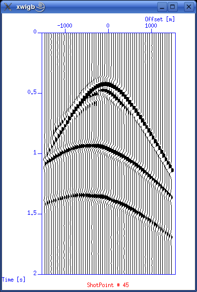
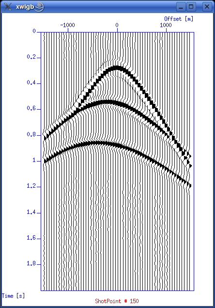
Display shot gather

This is exciting! We've just returned from the field with a brand new dataset. Let's first check trace headers used.

olem@seismix:~/www/course/> surange < seis.data
12000 traces:
tracl    1 12000 (1 - 12000)
tracr    1 12000 (1 - 12000)
fldr     1 200 (1 - 200)
tracf    1 60 (1 - 60)
trid     1
offset   -1475 1475 (-1475 - 1475)
sx       0 9950 (0 - 9950)
gx       -1475 11425 (-1475 - 11425)
ns       251
dt       8000

Then display shot gathers using this script from T. Benz' report:

#!/bin/sh

#------------------------------------------------
# Display of a SHOT gather between 1 and 200 
#------------------------------------------------

if [ $1 -le 200 ]; then
	if [ $1 -ge 1 ]; then
		suwind <seis.data key=fldr min=$1 max=$1 |
		suxwigb title="ShotPoint # $1" key=offset \
		label1="Time [s]" label2="Offset [m]" \
              	x2beg=-1500 x2end=1500 perc=95
	exit 0
	fi
fi

echo usage: showshot [shotpoint between 1 and 200]

exit

Save script to file showshot and make executable. Run by typing (now viewing shot gather no. 45):

./showshot 45

These are the shot gathers from SP=45 and SP=150. Compare them to plots in T. Benz report.

Fig. 6.2. Shot gather, SP=45.

Fig. 6.3. Shot gather, SP=150.

Near-trace plot

As mentioned in previous sections, a near-trace plot is very useful to get a first impression of data quality.

In our survey, shot positions are in the middle of the "geophone" layout - what is called "split-spread". With 60 "geophones", we can use no. 30 as near-trace. We extract traces from "geophone" no. 30 using the following command:

suwind key=tracf min=30 max=30 < seis.data | suximage perc=95

Remember the SURANGE listing we got from our dataset? The TRACF trace header parameter counts channels (or "geophones") in each shot.

This is the result. Compared to the layered earth image at the top of this section, it seems we're on the right track.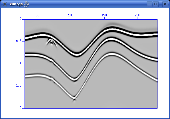

Fig. 6.4. Near-trace plot, channel no. 30.

PROCESSING SYNTHETIC DATA

We'll continue with processing of syntehic data aquired in the last section. We follow scripts in T. Benz report "Using Seismic Unix to Teach Seismic Processing".

Common-midpoint sorting

Common-midpoint sorting means selecting traces (from several shots) that share the same common midpoint, i.e. a hypothetical reflector midway between source and receiver.

Sorting method

Referring to T. Benz' report, ch. 4.2, this is the script that accomplishes the CMP sorting.

#! /bin/sh

#------------------------------------------------------
# Compute CMP trace header and sort data to CMP gathers
#------------------------------------------------------
suchw < seis.data key1=cdp key2=gx key3=sx \
                  a=1525 b=1 c=1 d=50 |
  susort > cmp.data cdp offset

exit 0

Copy and paste the script to a file called cmpsort.sh, make executable and run it.

A new Seismic Unix command is introduced - SUCHW - meaning "SU Change Header Word". The SUCHW applies the following operation (from SUCHW documentation):

     The value of header word key1 is computed from the values of key2 and key3 by:

        val(key1) = (a + b * val(key2) + c * val(key3)) / d

So the script uses the CDP header parameter as key1, GX (receiver coordinate) as key2 and SX (source coordinate) as key3. And we have a=1525 b=1 c=1 d=50, so we can then write:

       CDP = (1525 + GX + SX) / 50

If there's time we'll try to sketch the geometry in order to see how this expression works.

The output traces from the SUCHW command - now with the CDP trace header parameter set - are piped to a new command: SUSORT. As the name implies, SUSORT performs a sorting action, with two keys. The first key is CDP, and the next OFFSET.

What's the difference between CMP and CDP? CMP is simply the geometric midpoint between source and receiver. CDP stands for "Common Depth Point" and is often use instead of CMP. The problem is that dipping reflectors means there are no common depth points. So use of CDP should be avoided. But Seismic Unix uses CDP to denote what should really be called CMP.

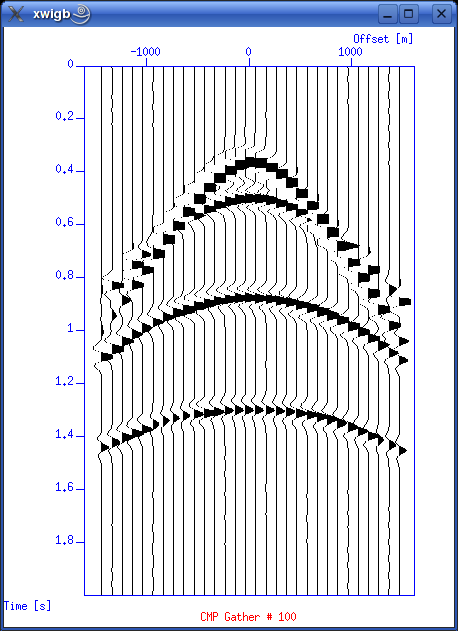
If we use SURANGE to examine the sorted traces, we notice the appearance of the CDP parameter, counting from 1 to 458:

   olem@seismix:~/www/course/ch4> surange < cmp.data
   12000 traces:
   tracl    1 12000 (1 - 12000)
   tracr    1 12000 (1 - 12000)
   fldr     1 200 (1 - 200)
   tracf    1 60 (1 - 60)
   cdp      1 458 (1 - 458)
   trid     1
   offset   -1475 1475 (-1475 - 1475)
   sx       0 9950 (0 - 9950)
   gx       -1475 11425 (-1475 - 11425)
   ns       251
   dt       8000

So we have more CMPs (458) that shotpoints (200). The reason is that distance between CMPs are half the distance between shotpoints. So there are fewer traces in a CMP gather then there are in a shot gather. At the ends of the survey line there are also CMPs with few traces.

Plotting CMP gathers

This scripts plots CMP gathers. Save as file showcmp.sh. Specify CMP number between 1 and 458.

#!/bin/sh

#------------------------------------------------
# Display of a CMP gather between 1 and 458
#------------------------------------------------

if [ $1 -le 458 ]; then
	if [ $1 -ge 1 ]; then
		suwind < cmp.data key=cdp min=$1 max=$1 |
		suxwigb title="CMP Gather # $1" key=offset \
		label1="Time [s]" label2="Offset [m]" \
		x2beg=-1500 x2end=1500 perc=95 \
		wbox=450 hbox=600
	exit 0
	fi
fi

echo usage: showcmp [gather between 1 and 458]

exit

Execute script:

    ./showcmp.sh 100 

The result should be like this.

Fig. 7.1. CMP gather no. 100

Fig. 7.2. CMP gather no. 300

Velocity analysis

The interactive velocity script is broken. The script was written several years ago and over time some of the commands used in the script may change type of input options. This is the case for the UNISAM program. It does not seem to accept file of x,y values in "par.uni" format - it will not generate an output file - so the next command will crash the script.

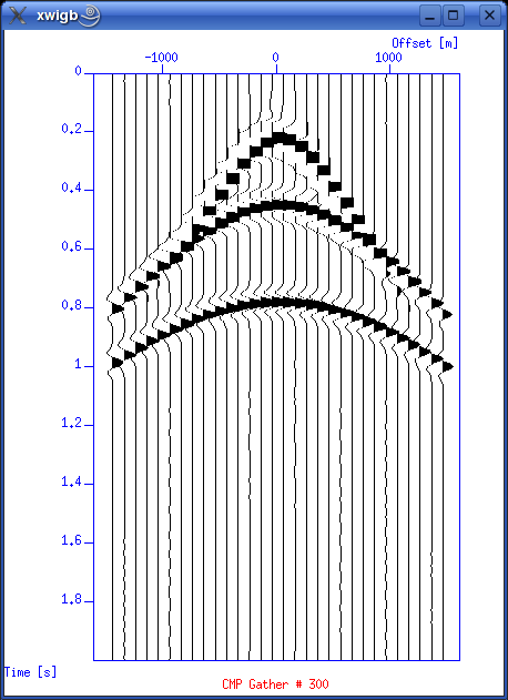
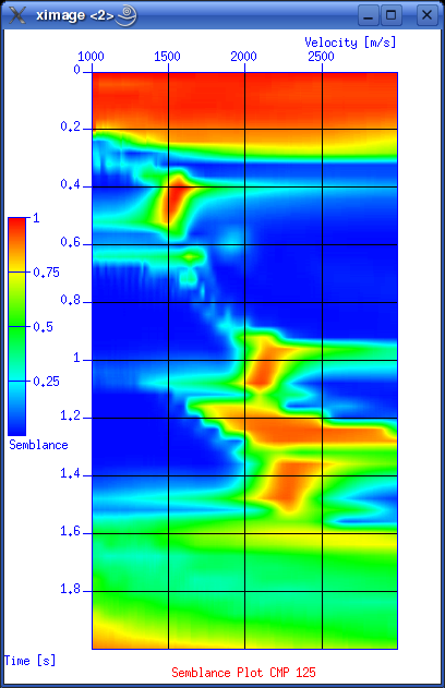
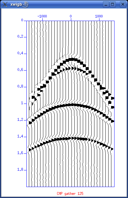
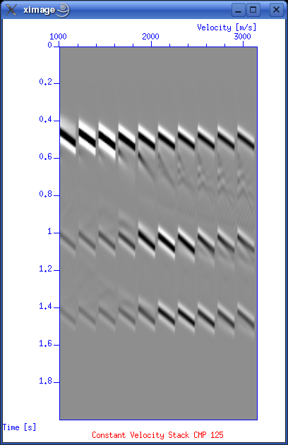
This is a reasonable advanced script that provide an interactive velocity picking session. It will first ask the user to input number of picks. You are then asked to state the CMP number for the first pick. After that it will make three plots:

• Semblance plot of the selected CMP number
• Plot of the selected CMP gather
• Constant Velocity Stack of the selected CMP number

#! /bin/sh

#set -x

#++++++++++++++++++++++++++++++++++++++++++++++++++++++++++++++++++++++++++++++++++++
#+++++++++++         W A R N I N G    --    W A R N I N G                   +++++++++
#+++++++++++                                                                +++++++++
#+++++++++++    Script will crash  - see comments in line 142               +++++++++
#++++++++++++++++++++++++++++++++++++++++++++++++++++++++++++++++++++++++++++++++++++

if [ ! -f cmp.data ]
then    echo "Sort to CMP first!"
        pause EXIT
        exit 
fi

echo "Velocity Analysis"

rm -f panel.* picks.* par.* tmp*

#------------------------------------------------
# Defining Variables etc...
#------------------------------------------------

indata=cmp.data
outdata=vpick.data

nt=251
dt=0.008

nv=200   # Number of Velocities
dv=10    # Interval
fv=1000  # First Velocity

>$outdata   # Write an empty file
>par.cmp    # Write an empty file

#------------------------------------------------
# Interactive Velocity Analysis...
#------------------------------------------------

echo "How many Picks? (typical 4)" >/dev/tty 
read nrpicks

i=1	
while [ $i -le $nrpicks ]
do
    echo "Specify CMP Pick Location (CMP gather number) $i" >/dev/tty 
    read picknow
    echo "Preparing Location $i of $nrpicks for Picking "
    echo "Location is CMP $picknow "

#------------------------------------------------
# CMP Gather Plot...
#------------------------------------------------

    suwind <$indata key=cdp min=$picknow \
            max=$picknow >panel.$picknow 
    suxwigb <panel.$picknow xbox=422 ybox=10 \
             wbox=400 hbox=600 \
             title="CMP gather $picknow" \
             perc=94 key=offset verbose=0 &

#------------------------------------------------
# Constant Velocity Stack (please wait)...
#------------------------------------------------

    >tmp1			# Create empty file
    j=1
    k=`expr $picknow + 10`
    l=`echo "$dv * $nv / 120" | bc -l`

	suwind < $indata key=cdp min=$picknow \
			max=$k > tmp0

    while [ $j -le 10 ]
    do
		vel=`echo "$fv + $dv * $j * $nv / 10" | bc -l`

		sunmo < tmp0 vnmo=$vel |
			sustack >> tmp1
		sunull ntr=2 nt=$nt dt=$dt >> tmp1
		j=`expr $j + 1`
    done

	suximage <tmp1 xbox=834 ybox=10 wbox=400 hbox=600 \
			title="Constant Velocity Stack CMP $picknow" \
			label1="Time [s]" label2="Velocity [m/s]" \
			f2=$fv d2=$l verbose=0 mpicks=picks.$picknow \
			perc=99 n2tic=5 cmap=rgb0 &		

#------------------------------------------------
# Semblance Plot...
#------------------------------------------------

	echo "  Place the cursor over the semblance plot or the"
	echo "  constant velocity stack and type 's' to pick velocities."
	echo "  For each suitable cursor position, press 's' to pick."
	echo "  Type 'q' in the semblance plot when all picks are made."
	echo "  A NMO corrected gather will be plotted after picking"

	suvelan < panel.$picknow nv=$nv dv=$dv fv=$fv |
		suximage xbox=10 ybox=10 wbox=400 hbox=600 \
			units="semblance" f2=$fv d2=$dv \
			label1="Time [s]" label2="Velocity [m/s]" \
			title="Semblance Plot CMP $picknow" cmap=hsv2 \
			legend=1 units=Semblance verbose=0 gridcolor=black \
			grid1=solid grid2=solid mpicks=picks.$picknow

	# Sort, using -n option -> "compare according to string numerical value"
	# Generate PAR file

	sort < picks.$picknow -n | mkparfile string1="tnmo" string2="vnmo" > par.$i

	cat par.$i
	echo "Completed listing of mkparfile output ..."


#------------------------------------------------
# NMO Plot and Velocity Profile...
#------------------------------------------------

	>tmp2				# Create empty file
	echo "cdp=$picknow" >> tmp2
	cat par.$i >> tmp2
	sunmo <panel.$picknow par=tmp2 |
		suxwigb title="CMP gather after NMO" xbox=10 ybox=10 \
				wbox=400 hbox=600 verbose=0 key=offset perc=94 &

	# SED info: http://www.grymoire.com/Unix/Sed.html
	cat par.$i | sed -e 's/tnmo/xin/' -e 's/vnmo/yin/' > par.uni.$i

	cat par.$i
	echo "Completed listing of par file A ..."
	cat par.uni.$i
	echo "Completed listing of par file B ..."

	# ------------  UNIformly SAMple a function y(x) specified as x,y pairs
	#++++++++++++++++++++++++++++++++++++++++++++++++++++++++++++++++++++++++++++++++++++
	#+++++++++++   W A R N I N G    ++++++    W A R N I N G    ++++++++++++++++++++++++++
	#++++++++++++++++++++++++++++++++++++++++++++++++++++++++++++++++++++++++++++++++++++
	# The UNISAM program does not seem to accept file of x,y in "par.uni" format.
	# It has probably been changed since the script was written several years ago.
	# So input to the UNISAM program must be corrected!
	# It will not generate an output file - so the next command will crash the script!!
	#++++++++++++++++++++++++++++++++++++++++++++++++++++++++++++++++++++++++++++++++++++

	unisam nout=$nt fxout=0.0 dxout=$dt par=par.uni.$i method=mono > tmp.unisam

	echo "Completed unisam command ..."

	cat tmp.unisam |
		 xgraph n=$nt nplot=1 d1=$dt f1=0.0 \
			label1="Time [s]" label2="Velocity [m/s]" \
			title="---> Stacking Velocity Function CMP $picknow" \
			-geometry 400x600+422+10 style=seismic \
			grid1=solid grid2=solid linecolor=3 marksize=1 mark=0 \
			titleColor=red axesColor=blue &

	echo "Picks OK? (y/n) " >  /dev/tty
	read response

	rm tmp*

	case $response in
		n*)
			i=$i
			echo "Picks removed"
			;;
		*)
			i=`expr $i + 1`
			echo "$picknow  $i" >> par.cmp
			;;
    esac
done

echo "Completed picking ..."

#------------------------------------------------
# Create Velocity Output File...
#------------------------------------------------

mkparfile < par.cmp string1=cdp string2=# > par.0

i=0
while [ $i -le $nrpicks ]
do
	cat par.$i >>$outdata
	i=`expr $i + 1`
done

rm -f panel.* picks.* par.* tmp*

exit

Corrections:

# Extract x- and y-values. Get rid of "xin=" and "yin=" line prefixes.

xval=`cat "par.uni.$i" | grep "xin=" | sed -e 's/xin=//'`
yval=`cat "par.uni.$i" | grep "yin=" | sed -e 's/yin=//'`
echo xval : $xval
echo yval : $yval

# Using Seimic Unix version 39 ... check. Only Y-values out??

unisam xin=$xval yin=$yval nout=$nt fxout=0.0 dxout=$dt method=mono > unisam.file
echo "Completed unisam command ..."

# Now plot with xgraph. Notice "pairs=2" since we only have y-values in input file.

xgraph pairs=2 n=$nt nplot=1 d1=$dt f1=0.0 \
	label1="Time [s]" label2="Velocity [m/s]" \
	title="---> Stacking Velocity Function CMP $picknow" \
	-geometry 400x600+422+10 style=seismic \
	grid1=solid grid2=solid linecolor=3 marksize=1 mark=0 \
	titleColor=red axesColor=blue < unisam.file &

These first three plots will look like:

Now start picking velocities in the semblance plot by first selecting the plot (click on upper border), then place cursor on pick points and press 's' for each point. When you are done press 'q' to quit. The script will then continue.

Normal moveout correction

Muting

Stacking

LINKS

These software packages can be evaluated. Thanks to J.O. Knutsen for providing the links.

Interpretation

• http://sourceforge.net/projects/javaseis (?)
• http://sourceforge.net/projects/gsegyview (Viewer?)
• http://sourceforge.net/projects/jpick
• http://www.kogeo.de/
• http://www2.opendtect.org/
• http://www.sciencedirect.com/science?_ob=ArticleURL&_udi=B6V7D-4F5S7W0-1&_user=10&_handle=V-WA-A-W-AV-MsSAYZA-UUW-U-AAWUWYWWYZ-AAADYZBUYZ-AVZZCUZEW-AV-U&_fmt=summary&_coverDate=06%2F30%2F2005&_rdoc=7&_orig=browse&_srch=%23toc%235840%232005%23999689994%23594428!&_cdi=5840&view=c&_acct=C000050221&_version=1&_urlVersion=0&_userid=10&md5=7275f2beed85334abb08063b0aaaccdc

Geomodelling / maps

• http://sourceforge.net/project/showfiles.php?group_id=129964
• http://sourceforge.net/projects/surfit
• http://sourceforge.net/projects/geoblock
• http://sourceforge.net/projects/gplates (Trond Torsvik et al)
• http://sourceforge.net/projects/fmesh

Seismics/processing

• ! http://sourceforge.net/projects/seismic-toolkit
• http://sourceforge.net/projects/gebr

Geostatistics

• http://sourceforge.net/projects/gstl

Raytracing

• http://sourceforge.net/projects/artsystem

Libraries

• http://sourceforge.net/projects/gplib

Other - check

• http://sourceforge.net/softwaremap/trove_list.php?form_cat=567
• "An open source, web based, simple solution for seismic data dissemination and collaborative research", by Paolo Diviacco

Seismic Unix (SU)

SU Home

Installation

Information