
|
Surveys and data Instruments
Support to other department sections Support Dr. Scient. thesis Contribution to "Scientific infrastructure"
Obsolete, kept for reference
Last update: April 30, 2025, at 08:49 AM |
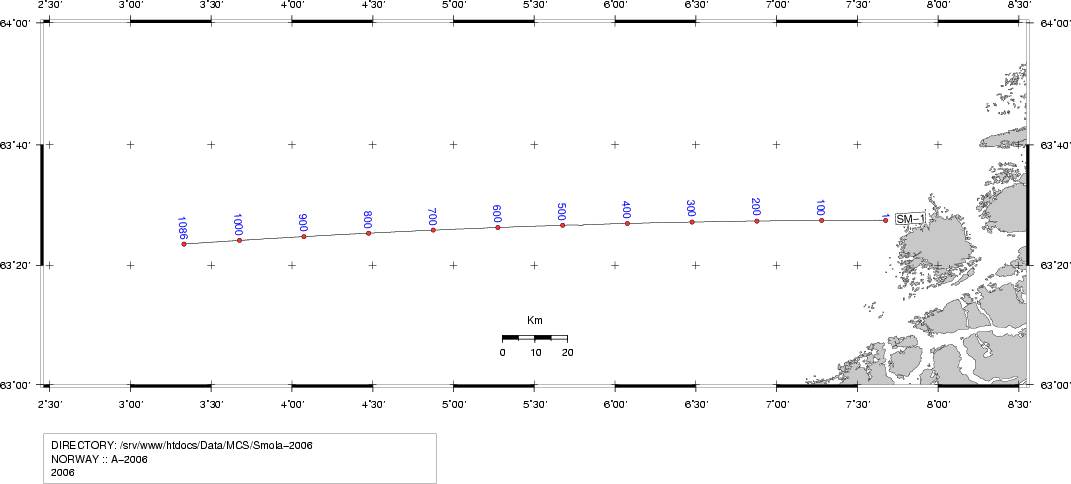 ABOUT THE SMØLA-2006 SURVEYThe Smøla-2006 survey was conducted 24/25 October 2006. RV "Håkon Mosby" was acting as source vessel for a land survey. Unfortunately, a GPS based unit that performs accurate time stamping of shot events was left behind. Time stamps are reconstructed as described below.
SMØLA-2006: RECONSTRUCTION OF SHOTPOINT TIMES
G. Landa, Instrumentation engineer, RV "Håkon Mosby", for performing measurements. B.O. Ruud, researcher IFG, for review and suggestions.
SUMMARYA linear time correction should be applied to the original time stamp values, from 6.95 s at SP=1 to 7.30 s at the last shotpoint. The correction should be subtracted from the original time stamp values. The UKOOA P1/90 file based on corrected shotpoint times can be downloaded from: Note that time stamp values are placed in columns 7 to 19 (normal GEOMAR positions). To re-generate UKOOA file with other time offset values, download these files to the same folder, make corrections in Python script, and execute script:
INTRODUCTIONUsing RV "Håkon Mosby", the Smøla line was shot from 10:19 UTC, 24. October 2006, and finished 24 hours later. The ship's airguns were used as source, and land stations recorded the seismic data. Accurate time stamping of shot events - to millisecond resolution - was thus of utmost importance. Unfortunately, the special GPS unit that performs the time stamping had earlier been used on another survey with RV "G.O. Sars" and left behind there. It could not be shipped to reach Mosby in time. Instead of cancelling the Smøla survey it was decided to carry on as planned, and post-process shotpoint time and positional data in order to achieve shotpoint time stamps of acceptable accuracy.
INSTRUMENTATIONFigure 1 shows the instrumentation system as it was supposed to be. Missing parts are at the bottom, below marker line.
Fig. 1: Smøla-2006 Instrumentation system (airguns omitted) Description of key instrument components
HOW TO RECONSTRUCT SHOTPOINT TIMESWhen trying to estimate time from positional information, one should keep in mind that uncertainties in positions translate into large (in our case) uncertainties in time. The ship moved at a speed of 5 knots, which is (1852*5)/(60*60) = 2.57 m/s. So positions that deviates from the true location by more then one meter result in nearly 0.4 s error in time. There are also some assumptions that must be made regarding drift in the Eiva Survey computer local clock. Should we apply a constant offset to Eiva timestamps in order to obtain true time (assuming zero clock drift), or is there a drift component, and how can it be determined? These matters are addressed below. There are some methods to estimate true shotpoint time stamp values.
Measurements were carried out with the aim of correcting shotpoint time according to Method B. Measurement were planned on 6. November 2006 - immediately after completion of the Smøla survey - but the shipment of the Ashtech GPS from the other research vessel did not reach Mosby in time. The measurements did not take place until March 2007. To further complicate matters, the EIVA Survey Computer had been switched off and on some times since the Smøla survey was completed. The complication lies in the fact that while PC's are furnished with battery-backed real-time clocks, the operating system usually only reads this clock in the power-up phase, and later on establishes its own internal clock based on another crystal - and hence shows a different time drift pattern, compared to that of the real-time clock crystal. Repeatedly switching the EIVA Survey computer off and on thus creates a clock problem that probably makes it impossible to use Method B. So we will in the following investigate Method A - interpolating 1-minute data from the Survey logger, and tie shotpoint locations to these interpolations. We will also use Method C to obtain information on time difference Eiva local clock and GPS time of those one-minute positions that are very close to a particular shotpoint.
DOWNLOAD LOGS, DATA
Combined data - both from EIVA Survey computer og Ashtech logger PC - which permits estimation of deviation (and it's drift) between EIVA PC local clock and true GPS time:
Thanks to G. Landa, Instrument Engineer on board RV "Håkon Mosby", for performing these measurements.
EMAIL LOGContact author if translation into English is needed.
PRE-PROCESSINGPreprocessing data from Survey logger - part 1
Download pre-processed data file. Preprocessing data from Survey logger - part 2The pre-processed file from previous section contains lines with several columns of data. We must extract time and position data, convert positions to UTM values and create two output files, one with Time/Easting data pairs, the other with Time/Northing pairs. The reason for this Easting/Northing split is that we must treat the two pairs separately in the subsequent interpolation stage. Time is also converted from a specific date/hour:minute etc. value to the number of seconds - with fractional part - since a reference base time set to midnight on 24. October 2006. Note that UTM values are given in zone 32V, whereas UTM coordinates in the shotpoint log are given in zone 31N; this is taken into account in later sections. The UTM/LatLong conversion is performed by a special library. Python script that extracts position/time from automatic survey logger machine. The two output files from the program can be downloaded from here:
METHOD A: INTERPOLATION OF TIME/POSITION VALUESTwo stages are needed. First interpolated values must be calculated. Then shotpoint positions must be tied to nearest interpolated position. Interpolation stageWe here employ a spline type of interpolation. Using the GNU spline command (on a Linux machine) results in an interpolated data set with user defined resolution. Our Time/Easting and Time/Northing files contains 1340 lines of 1-minute positions. To obtain 100x interpolation use -n 134000 option, and -n 134000 for 1000x interpolation. Command line example, on Linux machine: cat time_latitude.txt | spline -n 134000 -P 12 > spline-time_lat.txt Ensure that the number of significant digits in the calculations are sufficient (the -P option). As an illustration of how the spline interpolation works, figure 2 shows plot of latitude versus time. The 1-minute input values from the Survey logger are shown as red crosses, while the interpolated data pairs are green dots. The high interpolated data density (100 points between two original data pairs) makes them appear as a continuous line. Figure 3 zooms in on a section of the curve, making the individual interpolated data points visible. Figure 2 shows a small irregularity in the seismic line positioning. This is not uncommon, and was merely selected to show how the interpolation could cope. 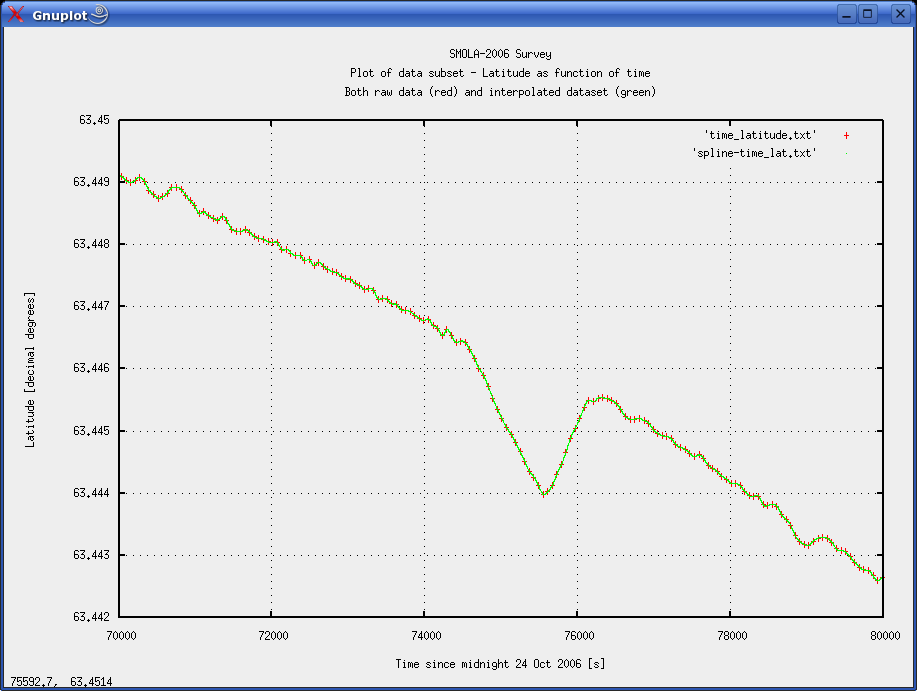 Fig. 2: Plot of latitude versus time. Original 1-minute data pairs as red crosses; interpolated data as green points. 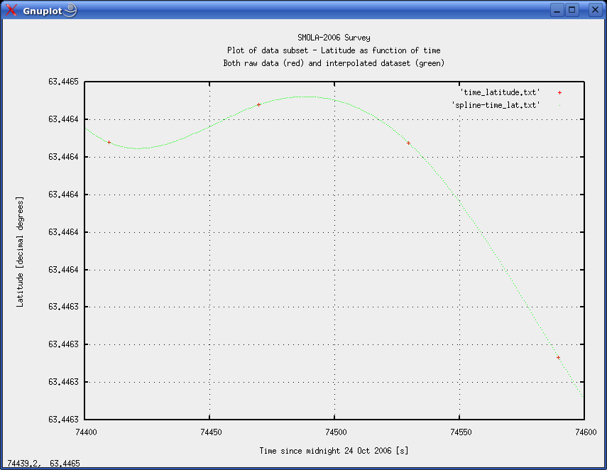 Fig. 3: Detail from figure 2. Individual interpolation points are now visible. We tried two different sizes of interpolation steps - both 100x and 1000x, to see how step size influenced the result.
Tie shotpoint to nearest interpolated locationThe following Python script ties the position of each shotpoint to interpolated values based on one-minute Survey logger data. Example of print-out from this script. Parameter description:
Download final result files: QC plot of results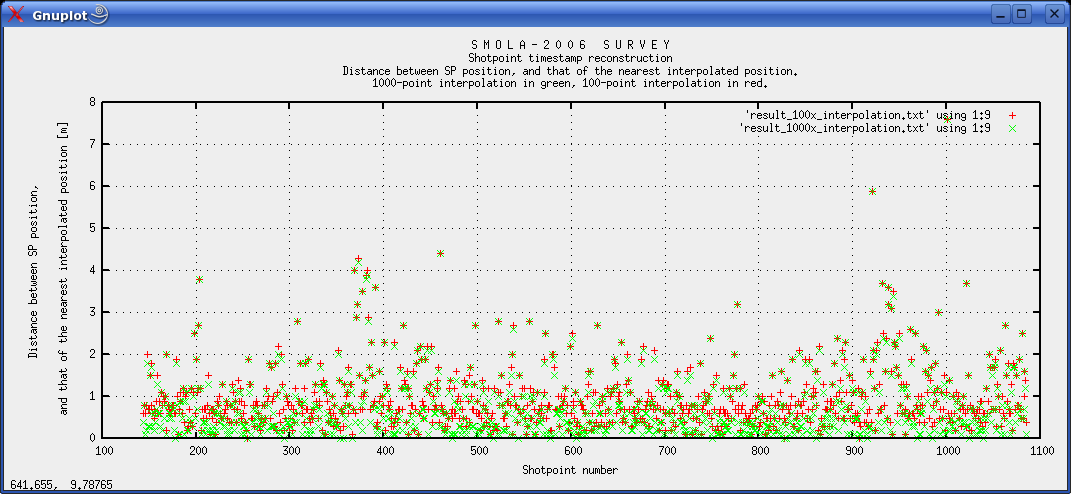 Fig. 4: Plot of distance between shotpoint and nearest interpolated position. 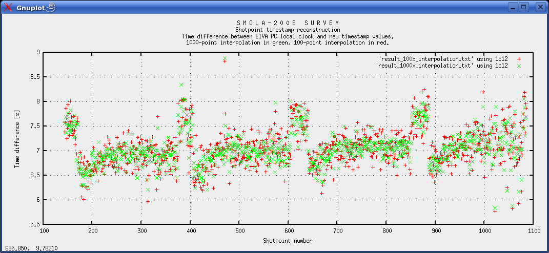 Fig. 5: Plot of time difference between original time stamps (EIVA Survey computer local clock), and new interpolated shotpoint times. Fig. 5 exhibits what at first view seems to be a strange periodicity. We believe the reason is the interference (or difference frequency) between shotpoint interval frequency, and one-minute position logging frequency, translated into the spatial (easting/northing) domain. When shotpoints are far from one-minute positions the interpolation has the lowest accuracy. Due to the interference, there are small regions of shotpoints that are far from one-minute positions. It is not likely that the Eiva computer local clock should have a drift pattern as shown in fig. 5. So when estimating time correction values from fig. 5 one should disregard the peaks and lows of the curve, and instead place a straight line through the stable intervals (follow the back of the "horses"). It appears that the delay increases from around 6.95 s in the start, to 7.3 at the end. We assume that the Eiva PC local clock has a linear time drift pattern. Around 0.3 seconds per day seems to be a reasonable figure. Fig. 6 illustrates that the interpolated curve does not necessarily pass through all shotpoints. This explains why there can be a distance of several meters between a particular shotpoint, and the nearest interpolated point. 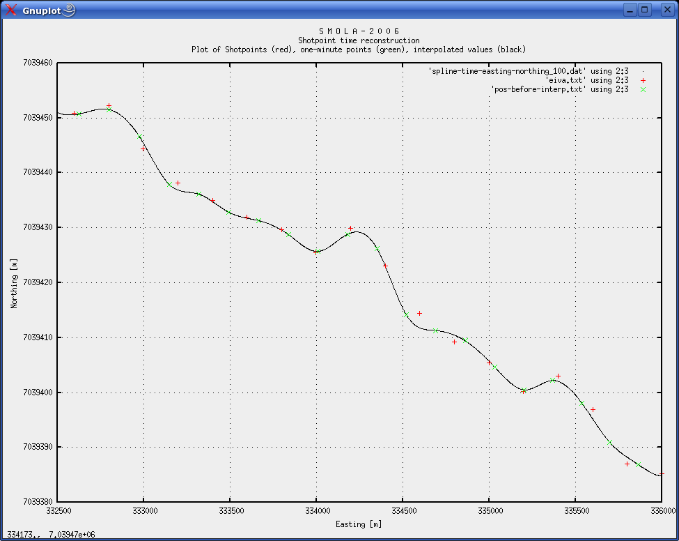 Fig. 6: Plot of Shotpoints, one-minute positions and interpolated positions.
METHOD C: SHOTPOINTS THAT MATCH POSITIONS IN ONE-MINUTE FILESThis Python script will search the one-minute file for positions that are within a user-defined distance from the shotpoints. The distance limit is set to 1 m. Remember what was mentioned in the beginning: A 1 m distance uncertainty translates into approx 0.4 s time uncertainty (assuming 5 kt ship speed). The results - for 1 m distance limit - are presented below. Parameter explanation:
  Column no:    Description
           1 :  EIVA SP
           2 :  EIVA Easting
           3 :  EIVA Northing
           4 :  EIVA Date
           5 :  EIVA Time
           6 :  One-min Easting
           7 :  One-min Northing
           8 :  One-min Date
           9 :  One-min Time
          10 :  Delta distance
          11 :  Delta time
000196 394979.08 7038165.61 2006-10-24 14:50:16.843000 394979.66 7038165.86 2006-10-24 14:50:09.970000 0.63 0:00:06.873000
000249 384384.46 7038386.68 2006-10-24 15:54:17.406000 384383.57 7038386.62 2006-10-24 15:54:10.740000 0.89 0:00:06.666000
000298 374588.65 7038593.12 2006-10-24 16:53:17.703000 374588.79 7038592.71 2006-10-24 16:53:10.540000 0.43 0:00:07.163000
000552 323799.10 7039643.70 2006-10-24 22:36:17.734000 323799.90 7039643.77 2006-10-24 22:36:10.340000 0.80 0:00:07.394000
000847 264787.21 7040850.75 2006-10-25 04:44:18.359000 264787.56 7040850.79 2006-10-25 04:44:11.050000 0.35 0:00:07.309000
000888 256583.92 7041035.54 2006-10-25 05:36:17.718000 256584.06 7041034.83 2006-10-25 05:36:10.870000 0.72 0:00:06.848000
000940 246178.26 7041239.36 2006-10-25 06:45:17.703000 246177.97 7041239.61 2006-10-25 06:45:10.630000 0.38 0:00:07.073000
001002 233770.89 7041492.60 2006-10-25 08:10:18.859000 233771.59 7041492.38 2006-10-25 08:10:11.330000 0.73 0:00:07.529000
001031 227967.15 7041621.67 2006-10-25 08:51:18.203000 227966.31 7041621.58 2006-10-25 08:51:11.190000 0.84 0:00:07.013000
A 0.5 m distance limit yields these matches: 000298 374588.65 7038593.12 2006-10-24 16:53:17.703000 374588.79 7038592.71 2006-10-24 16:53:10.540000 0.43 0:00:07.163000 000847 264787.21 7040850.75 2006-10-25 04:44:18.359000 264787.56 7040850.79 2006-10-25 04:44:11.050000 0.35 0:00:07.309000 000940 246178.26 7041239.36 2006-10-25 06:45:17.703000 246177.97 7041239.61 2006-10-25 06:45:10.630000 0.38 0:00:07.073000 Of the last three matches that are within 0.5 m, we have time deltas of 7.163, 7.309 and 7.073 s. As a further aid in determining the time difference, we plot these three shotpoints, together with corresponding positions from one-minute file:  Fig. 7: Plot of SP=298, and corresponding position in one-minute file. DeltaD: 0.43 m, DeltaT: 7.163 s. 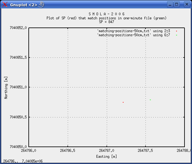 Fig. 8: Plot of SP=847, and corresponding position in one-minute file. DeltaD: 0.35 m, DeltaT: 7.309 s.  Fig. 9: Plot of SP=940, and corresponding position in one-minute file. DeltaD: 0.38 m, Delta t = 7.073 s. There is an important observation to be made. In fig. 7 and 8, the shotpoint occurs AFTER the corresponding one-minute position, while in fig. 9, it occurs BEFORE the one-minute position. This is because the line was traversed from EAST to WEST. So in the latter case, the time difference should be SMALLER then in the two first cases - and this is supported by the data. So the true time delay should be between 7.073 and a time represented by the two other figures - 7.309 and 7.163 s. For the moment, let's concentrate on shotpoint pairs 847 and 940 that are near symmetrical on either side of corresponding one-minute positions. They are only two hours apart, so drift in Eiva local clock should be minimal. For SP=847 we have 0.35m/7.309s, and for SP=940 we have 0.38m/7.073s. To strengthen our argument, let's calculate how long it takes to travel 0.35 and 0.38 m, assuming ship's speed was 5 kt (2.57 m/s):
     Time to travel 35 cm @ 5 kt: 35/257 = 0.136 s
     Time to travel 38 cm @ 5 kt: 38/257 = 0.148 s
As SP=847 and SP=940 is symmetrical on each side of one-minute positions, the time difference - estimated from ship's speed alone - should be 0.136+0.148 = 0.284 s. Compare this to the difference between times that were observed for the two symmetrical shotpoints 847 and 940: 7.309 - 7.073 = 0.236 s. Let's choose 0.250 s as the time difference between these two symmetrical shotpoints. So for SP=847, we should subtract 0.250*(35/(35+38)) = 0.120 s, yielding 7.309 - 0.120 = 7.209 s. For SP=940, we should add 0.250*(38/(35+38)), yielding 7.073 + 0.130 = 7.203. From this we estimate that there is a time difference of 7.2 s between EIVA local clock time stamps, and true UTC time. This value should be subtracted from the EIVA values. This conclusion was based on data from two shotpoints, two hours apart. Let's check all shotpoints that lies less then 1 m from one-minute point.
Time @ 5 kt: 1/(1852*5/3600) * Delta distance. Add/subtract: If SP Easting is lower then one-min Easting, SP occurred AFTER one-min position. In that case, add. Note 1): Position mainly changes in N-S direction. Discard. The figures in the "Result" column suggest that there is a slight drift in the Eiva local clock during the time the line was shot. We could linearly apply 6.95 s correction for the first SP, and 7.30 for the last. This yields 0.35 s drift during the 24 hours it took to shoot the line. The drift in time adjustment values can be seen in the figure below. 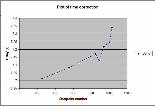 Fig. 11: Plot of time correction as function of shotpoint. Disregarding outliers at SP=888 and 1031, and placing a straight line through the remaining points, one should have 6.95 s correction at SP=1 and 7.3 s correction at the last SP.
PROGRAM FOR TIME CORRECTION, UKOOA GENERATIONThe following Python script performs:
The output files are here: Plot of original (red) and adjusted (green) shotpoint positions illustrates how the vector based offset method works. A spline interpolation is probably more appropriate, but the increased precision is not deemed necessary. The vector based method is simple - spline interpolation requires a lot more programming effort, and the gain is marginal ... 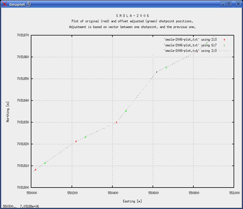 Fig. 12: Plot of original (red) and offset adjusted (green) shotpoint positions, illustrating the effect of vector based offset method.
APPENDIX: GNUPLOT COMMANDSset grid set xlabel "Time since midnight 24 Oct 2006 [s]" set ylabel "Latitude [decimal degrees]" set title "SMOLA-2006 Survey\nPlot of data subset - Latitude as function of time\nBoth raw data (red) and interpolated dataset (green)" plot 'time_latitude.txt' with points pt 1, 'spline-time_lat.txt' with points pt 0 set xrange [74000:76000] replot set xrange [70400:84600] replot QC-plots: set grid set xlabel "Shotpoint number" set ylabel "Distance between SP position,\n and that of the nearest interpolated position [m]" set title "S M O L A - 2 0 0 6 S U R V E Y\nShotpoint timestamp reconstruction\nDistance between SP position, \\ and that of the nearest interpolated position.\n1000-point interpolation in green, 100-point interpolation in red." plot 'result_100x_interpolation.txt' using 1:9 with points lt 1, 'result_1000x_interpolation.txt' using 1:9 with points lt 2 set ylabel "Time difference [s]" set title ""S M O L A - 2 0 0 6 S U R V E Y\nShotpoint timestamp reconstruction\nTime difference between EIVA PC local clock and new timestamp values" plot 'result_100x_interpolation.txt' using 1:12 with points lt 1, 'result_1000x_interpolation.txt' using 1:12 with points lt 2 replot |
||||||||||||||||||||||||||||||||||||||||||||||||||||||||||||||||||||||||||||||||||||||||||||